R, Python 분석과 프로그래밍의 친구 (by R Friend)

데이터 분석을 하다보면 데이터 전처리 단계에서 '결측값 확인 및 처리(handling missing values) '가 필요합니다.

시계열 데이터의 결측값을 처리하는 방법에는 보간(interpolation), 이전/이후 값으로 대체, 이동평균(moving average)으로 대체 등 여러가지 방법(https://rfriend.tistory.com/682)이 있습니다.

이번 포스팅에서는 가장 간단한 방법으로서 PostgreSQL, Greenplum DB에서 SQL로 first_value() window function을 사용해서 할 수 있는 '결측값을 이전 값으로 채우기' 또는 '결측값을 이후 값으로 채이기' 하는 방법을 소개하겠습니다. 

(1) 결측값을 이전 값으로 채우기

     (Forward filling NULL values with the previous non-null value)

(2) 여러개 칼럼의 결측값을 이전 값으로 채우기

     (Forward filling NULL values in Multiple Columns with the previous non-null value)

(3) 그룹별로 결측값을 이전 값으로 채우기 

     (Forward filling NULL values by Group with the previous non-null value)

(4) 결측값을 이후 값으로 채우기 

     (Backward filling NULL values with the next non-null value)

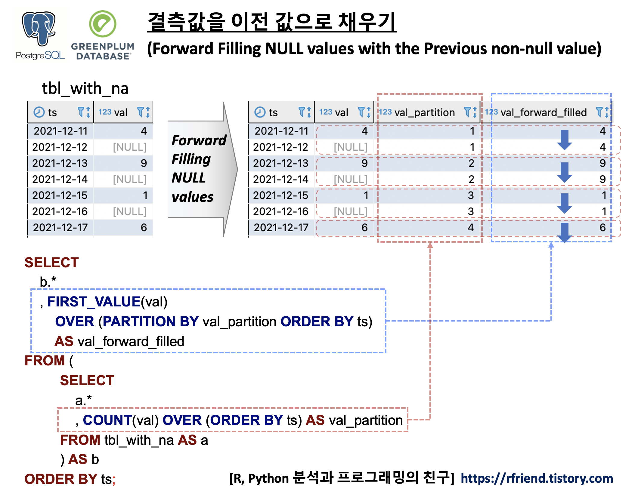
결측값을 시계열데이터의 TimeStamp 를 기준으로 정렬한 상태에서 SQL로 결측값을 이전의 실측값으로 채우는 방법의 핵심은 FIRST_VALUE() Window Function 을 사용하는 것입니다. FIRST_VALUE() 의 구문은 아래와 같으며, OVER(PARTITION BY column_name ORDER BY TimeStamp_column_name) 의 기능은 위의 예제에 대한 도식의 빨강, 파랑 박스와 화살표를 참고하시기 바랍니다. 

-- PostgreSQL FIRST_VALUE() Window Function syntax

FIRST_VALUE ( expression )  
OVER ( 
    [PARTITION BY partition_expression, ... ]
    ORDER BY sort_expression [ASC | DESC], ...
)

(1) 결측값을 이전 값으로 채우기

     (Forward filling NULL values with the previous non-null value)

먼저, 날짜를 나타내는 'ts' 칼럼과 결측값을 가지는 'val' 칼럼으로 구성된 예제 테이블을 만들어보겠습니다. 

-- creating a sample dataset with NULL values
DROP TABLE IF EXISTS tbl_with_na;
CREATE TABLE tbl_with_na (
	ts DATE NOT NULL
	, val int
);

INSERT INTO tbl_with_na VALUES 
('2021-12-11', 4)
, ('2021-12-12',NULL)
, ('2021-12-13', 9)
, ('2021-12-14', NULL)
, ('2021-12-15', 1)
, ('2021-12-16', NULL)
, ('2021-12-17', 6)
;

SELECT * FROM tbl_with_na ORDER BY ts;

--ts        |val|
------------+---+
--2021-12-11|  4|
--2021-12-12|   |
--2021-12-13|  9|
--2021-12-14|   |
--2021-12-15|  1|
--2021-12-16|   |
--2021-12-17|  6|

이제 FIRST_VALUE() OVER(), COUNT() OVER() 의 window function 을 사용해서 결측값을 이전 실측값으로 채워보겠습니다. 

-----------------------------------------------------
-- (1) Forward Filling NULL values
-----------------------------------------------------
SELECT 
	b.*
	, FIRST_VALUE(val) 
		OVER (PARTITION BY val_partition ORDER BY ts) 
			AS val_forward_filled
FROM (
	SELECT 
		a.*
		, count(val) OVER (ORDER BY ts) AS val_partition
	FROM tbl_with_na AS a
	) AS b
ORDER BY ts;

--ts        |val|val_partition|val_forward_filled|
------------+---+-------------+------------------+
--2021-12-11|  4|            1|                 4|
--2021-12-12|   |            1|                 4|
--2021-12-13|  9|            2|                 9|
--2021-12-14|   |            2|                 9|
--2021-12-15|  1|            3|                 1|
--2021-12-16|   |            3|                 1|
--2021-12-17|  6|            4|                 6|

(2) 여러개 칼럼의 결측값을 이전 값으로 채우기

     (Forward filling NULL values in Multiple Columns with the previous non-null value)

먼저, 날짜를 나타내는 칼럼 'ts'와 측정값을 가지는 2개의 칼럼 'val_1', 'val_2'로 구성된 예제 테이블을 만들어 보겠습니다. 

-- creating a sample table with NULL values in multiple columns
DROP TABLE IF EXISTS tbl_with_na_mult_cols;
CREATE TABLE tbl_with_na_mult_cols (
	ts DATE NOT NULL
	, val_1 int
	, val_2 int
);

INSERT INTO tbl_with_na_mult_cols VALUES 
('2021-12-11', 1, 5)
, ('2021-12-12',NULL, NULL)
, ('2021-12-13', 2, 6)
, ('2021-12-14', NULL, 7)
, ('2021-12-15', 3, NULL)
, ('2021-12-16', NULL, NULL)
, ('2021-12-17', 4, 8)
;

SELECT * FROM tbl_with_na_mult_cols ORDER BY ts;

--ts        |val_1|val_2|
------------+-----+-----+
--2021-12-11|    1|    5|
--2021-12-12|     |     |
--2021-12-13|    2|    6|
--2021-12-14|     |    7|
--2021-12-15|    3|     |
--2021-12-16|     |     |
--2021-12-17|    4|    8|

다음으로 결측값을 채우려는 여러개의 각 칼럼마다 FIRST_VALUE() OVER(), COUNT() OVER() 의 window function 을 사용해서 결측값을 이전 값으로 채워보겠습니다. 

------------------------------------------------------------------
-- (2) Forward Filling NULL values in Multiple Columns
------------------------------------------------------------------
SELECT 
	b.ts
	, b.val_1
	, b.val_1_partition
	, FIRST_VALUE(val_1) 
		OVER (PARTITION BY val_1_partition ORDER BY ts) 
		AS val_1_fw_filled
	, b.val_2
	, b.val_2_partition
	, FIRST_VALUE(val_2) 
		OVER (PARTITION BY val_2_partition ORDER BY ts) 
		AS val_2_fw_filled
FROM (
	SELECT 
		a.*
		, count(val_1) OVER (ORDER BY ts) AS val_1_partition
		, count(val_2) OVER (ORDER BY ts) AS val_2_partition
	FROM tbl_with_na_mult_cols AS a
	) AS b
ORDER BY ts;

--ts        |val_1|val_1_partition|val_1_fw_filled|val_2|val_2_partition|val_2_fw_filled|
------------+-----+---------------+---------------+-----+---------------+---------------+
--2021-12-11|    1|              1|              1|    5|              1|              5|
--2021-12-12|     |              1|              1|     |              1|              5|
--2021-12-13|    2|              2|              2|    6|              2|              6|
--2021-12-14|     |              2|              2|    7|              3|              7|
--2021-12-15|    3|              3|              3|     |              3|              7|
--2021-12-16|     |              3|              3|     |              3|              7|
--2021-12-17|    4|              4|              4|    8|              4|              8|

(3) 그룹별로 결측값을 이전 값으로 채우기 

     (Forward filling NULL values by Group with the previous non-null value)

이번에는 2개의 그룹('a', 'b')이 있고, 'val' 칼럼에 결측값이 있는 예제 데이터 테이블을 만들어보겠습니다. 

-- creating a sample dataset with groups
DROP TABLE IF EXISTS tbl_with_na_grp;
CREATE TABLE tbl_with_na_grp (
	ts DATE NOT NULL
	, grp TEXT NOT NULL
	, val int
);

INSERT INTO tbl_with_na_grp VALUES 
('2021-12-11', 'a',1) -- GROUP 'a'
, ('2021-12-12','a', NULL)
, ('2021-12-13', 'a', 2)
, ('2021-12-14', 'a', NULL)
, ('2021-12-15', 'a', 3)
, ('2021-12-16', 'a', NULL)
, ('2021-12-17', 'a', 4)
, ('2021-12-11', 'b', 11) -- GROUP 'b'
, ('2021-12-12', 'b', NULL)
, ('2021-12-13', 'b', 13)
, ('2021-12-14', 'b', NULL)
, ('2021-12-15', 'b', 15)
, ('2021-12-16', 'b', NULL)
, ('2021-12-17', 'b', 17)
;

SELECT * FROM tbl_with_na_grp ORDER BY grp, ts;

--ts        |grp|val|
------------+---+---+
--2021-12-11|a  |  1|
--2021-12-12|a  |   |
--2021-12-13|a  |  2|
--2021-12-14|a  |   |
--2021-12-15|a  |  3|
--2021-12-16|a  |   |
--2021-12-17|a  |  4|
--2021-12-11|b  | 11|
--2021-12-12|b  |   |
--2021-12-13|b  | 13|
--2021-12-14|b  |   |
--2021-12-15|b  | 15|
--2021-12-16|b  |   |
--2021-12-17|b  | 17|

이제 그룹 별로(OVER (PARTITION BY grp, val_partition ORDER BY ts)) 이전 값으로 채우기(FIRST_VALUE(val))를 해보겠습니다. 

----------------------------------------------------------
-- (3) Forward Filling NULL values by Group
----------------------------------------------------------
SELECT 
	b.*
	, FIRST_VALUE(val) 
		OVER (PARTITION BY grp, val_partition ORDER BY ts) 
		AS val_filled
FROM (
	SELECT 
		a.*
		, count(val) 
			OVER (PARTITION BY grp ORDER BY ts) 
			AS val_partition
	FROM tbl_with_na_grp AS a
	) AS b
ORDER BY grp, ts;

--ts        |grp|val|val_partition|val_filled|
------------+---+---+-------------+----------+
--2021-12-11|a  |  1|            1|         1|
--2021-12-12|a  |   |            1|         1|
--2021-12-13|a  |  2|            2|         2|
--2021-12-14|a  |   |            2|         2|
--2021-12-15|a  |  3|            3|         3|
--2021-12-16|a  |   |            3|         3|
--2021-12-17|a  |  4|            4|         4|
--2021-12-11|b  | 11|            1|        11|
--2021-12-12|b  |   |            1|        11|
--2021-12-13|b  | 13|            2|        13|
--2021-12-14|b  |   |            2|        13|
--2021-12-15|b  | 15|            3|        15|
--2021-12-16|b  |   |            3|        15|
--2021-12-17|b  | 17|            4|        17|

(4) 결측값을 이후 값으로 채우기 

     (Backward filling NULL values with the next non-null value)

결측값을 이전 값(previous non-null value)이 아니라 이후 값(next non-null value) 으로 채우려면 (1)번의 SQL 코드에서 OVER (ORDER BY ts DESC)) 처럼 내림차순으로 정렬(sorting in DESCENDING order) 해준 후에 FIRST_VALUE() 를 사용하면 됩니다. 

-----------------------------------------------------
-- (4) Backward Filling NULL values
-----------------------------------------------------

SELECT 
	b.*
	, FIRST_VALUE(val) 
		OVER (PARTITION BY grp, val_partition ORDER BY ts DESC) 
		AS val_filled
FROM (
	SELECT 
		a.*
		, count(val) 
			OVER (PARTITION BY grp ORDER BY ts DESC) 
			AS val_partition
	FROM tbl_with_na_grp AS a
	) AS b
ORDER BY grp, ts;

--ts        |grp|val|val_partition|val_filled|
------------+---+---+-------------+----------+
--2021-12-11|a  |  1|            4|         1|
--2021-12-12|a  |   |            3|         2|
--2021-12-13|a  |  2|            3|         2|
--2021-12-14|a  |   |            2|         3|
--2021-12-15|a  |  3|            2|         3|
--2021-12-16|a  |   |            1|         4|
--2021-12-17|a  |  4|            1|         4|
--2021-12-11|b  | 11|            4|        11|
--2021-12-12|b  |   |            3|        13|
--2021-12-13|b  | 13|            3|        13|
--2021-12-14|b  |   |            2|        15|
--2021-12-15|b  | 15|            2|        15|
--2021-12-16|b  |   |            1|        17|
--2021-12-17|b  | 17|            1|        17|

[ Reference ]

* PostgreSQL window function first_value()

  : https://www.postgresqltutorial.com/postgresql-first_value-function/

* PostgreSQL window functions

  : https://www.postgresql.org/docs/9.4/functions-window.html

이번 포스팅이 많은 도움이 되었기를 바랍니다. 

행복한 데이터 과학자 되세요!  :-)

지난번 포스팅에서는 PostgreSQL, Greenplum DB에서 옆으로 넓은 테이블(horizontally wide-format table)을 세로로 긴 테이블(vertically long-format table)로 변환(transpose)하는 2가지 방법을 소개하였습니다. (https://rfriend.tistory.com/713)

이번 포스팅에서는 반대로, PostgreSQL, Greenplum DB에서 세로로 긴 테이블을 가로로 넓은 테이블로 Pivot 하는 방법(Pivoting table, converting long-format table to wide-format table)을 소개하겠습니다. 보통 탐색적 데이터 분석, 통계 분석, 기계학습 등의 분석을 할 때는 pivot table 한 후의 각 ID별로 여러개의 칼럼이 옆으로 넓게 붙은 형태의 테이블을 사용합니다. 

* PostgreSQL과 Greenplum 에서 각각 다른 함수를 사용하는 것에 유의하세요. 

(1) PostgreSQL에서 tablefunc extension의 crosstab() 함수를 이용해 테이블 피봇하기

     (Pivoting table using crosstab() function in PostgreSQL)

(2) Greenplum 에서 Apache MADlib의 pivot() 함수를 이용해 테이블 피봇하기

     (Pivoting table using Apache MADlib's pivot() function in Greenplum)

(3) Manual 하게 Select 후 Join 해서 테이블 피봇하기 

     (Pivoting table by select and join manually) 

먼저, 예제로 사용할 간단한 예제 테이블을 만들어보겠습니다. 학생 ID별로 과목(class_nm) 별 점수(score) 를 저장해놓은 테이블입니다. 

--------------------------------------------------------------------------------
-- Pivoting table using crosstab() function in PostgreSql 9.4+
-- [ref] https://www.postgresql.org/docs/9.4/tablefunc.html
-- [ref] https://learnsql.com/blog/creating-pivot-tables-in-postgresql-using-the-crosstab-function/
--------------------------------------------------------------------------------

DROP TABLE IF EXISTS score_long;
CREATE TABLE score_long (
	id int NOT null
	, class_nm TEXT 
	, score int
);

INSERT INTO score_long VALUES 
 (1,'english' , 100)
, (1,'korean' , 100)
, (1,'math', 100)
, (2,'english', 75)
, (2,'korean', 80)
, (2,'math', 85)
, (3,'english', 98)
, (3,'korean' , 100)
, (3,'math', 60)
, (4,'english', 75)
, (4,'korean', 80)
, (4,'math', 98)
;

SELECT * FROM score_long ORDER BY id, class_nm;
--id|class_nm|score
----+--------+-----+
-- 1|english |  100|
-- 1|korean  |  100|
-- 1|math    |  100|
-- 2|english |   75|
-- 2|korean  |   80|
-- 2|math    |   85|
-- 3|english |   98|
-- 3|korean  |  100|
-- 3|math    |   60|
-- 4|english |   75|
-- 4|korean  |   80|
-- 4|math    |   98|

(1) PostgreSQL에서 tablefunc extension의 crosstab() 함수를 이용해 테이블 피봇하기

     (Pivoting table using crosstab() function in PostgreSQL)

세로로 긴 테이블을 가로로 넓은 테이블로 pivot 할 때 사용되는 crosstab() 함수는 PostgreSQL 버전 8.3 이 배포되었을 때 처음 소개되었던 tablefunc extension 에 포함되었습니다. 따라서 tablefunc extension 을 처음 사용하는 경우라면

CREATE EXTENSION tablefunc; 로 활성화시켜준 후에 crosstab() 함수를 호출해서 사용할 수 있습니다. 

crosstab() 함수는 SELECT 문의 FROM 절에 사용이 되므로 처음 사용하는 분이라면 좀 낯설게 여길 수도 있겠습니다. crosstab() 함수에서 SELECT 문은 3개의 칼럼을 반환합니다. 

(칼럼 1) 첫번째 칼럼은 각 관측치를 구분하는 ID (identifier) 칼럼입니다. 위의 예에서는 학생들의 ID가 이에 해당합니다. 

(칼럼 2) 두번째 칼럼은 pivot table 에서의 범주(categories)에 해당하는 칼럼입니다. pivot을 하게 되면 각 칼럼으로 변환이 됩니다. 위의 예에서는 과목명(class_nm) 칼럼이 이에 해당합니다. 

(칼럼 3) 세번째 칼럼은 pivot table 의 각 셀에 할당이 될 값(value)에 해당하는 칼럼입니다. 위의 예에서는 점수(score) 칼럼이 이에 해당합니다. 

crosstab() 함수안에 SQL query로 위의 3개 칼럼을 select 한 결과를, AS final_result() 에서 pivot table 에서 재표현할 칼럼 이름과 데이터 유형을 정의해주면 됩니다. 

-- (1) Pivoting table using PostgreSQL's crosstab() function
-- Enabling the Crosstab Function
-- : The crosstab() function is part of a PostgreSQL extension called tablefunc. 
CREATE EXTENSION tablefunc;

-- Pivoting table
--: The crosstab() function receives an SQL SELECT command as a parameter.
SELECT *
FROM 
	crosstab(
		'select id, class_nm, score 
		from score_long 
		order by 1, 2') 
	AS final_result(id int, english_score int, korean_score int, math_score int);

--id|english_score|korean_score|math_score|
----+-------------+------------+----------+
-- 1|          100|         100|       100|
-- 2|           75|          80|        85|
-- 3|           98|         100|        60|
-- 4|           75|          80|        98|

(2) Greenplum 에서 Apache MADlib의 pivot() 함수를 이용해 테이블 피봇하기

     (Pivoting table using Apache MADlib's pivot() function in Greenplum)

Greenplum 에서는 PostgreSQL에서 사용했던 crosstab() 함수를 사용할 수 없습니다 대신 Greenplum 에서는 테이블을 pivot 하려고 할 때 Apache MADlib의 pivot() 함수를 사용합니다. 아래의 madlib.pivot() 함수 안의 구문(syntax)을 참고해서 각 매개변수 항목에 순서대로 입력을 해주면 됩니다. 

--------------------------------------------------------------------------------
-- Pivoting table using crosstab() function in Greenplum
-- [ref] https://madlib.apache.org/docs/latest/group__grp__pivot.html
--------------------------------------------------------------------------------

-- Pivoting table using Apache MADlib's pivot() function

DROP TABLE IF EXISTS score_pivot;
SELECT madlib.pivot(
	'score_long' 		-- source_table,
	, 'score_pivot' 	-- output_table,
	, 'id' 					-- index,
	, 'class_nm' 		-- pivot_cols,
	, 'score' 			-- pivot_values,
	, 'avg' 				-- aggregate_func,
	, 'NULL'			-- fill_value,
	, 'False'			-- keep_null,
);


SELECT * FROM score_pivot ORDER BY id;
--id|score_avg_class_nm_english|score_avg_class_nm_korean|score_avg_class_nm_math|
--+--------------------------+-------------------------+-----------------------+
-- 1|      100.0000000000000000|     100.0000000000000000|   100.0000000000000000|
-- 2|       75.0000000000000000|      80.0000000000000000|    85.0000000000000000|
-- 3|       98.0000000000000000|     100.0000000000000000|    60.0000000000000000|
-- 4|       75.0000000000000000|      80.0000000000000000|    98.0000000000000000|

칼럼 이름이 자동으로 설정('피봇값_집계함수_카테고리 칼럼이름' 형식)이 되는데요, 만약 칼럼 이름을 사용자의 입맛에 맞게 새로 바꿔주고 싶으면 ALTER TABLE table_name RENAME COLUMN old_column TO new_column; 을 사용해서 바꿔주세요. 

-- Renaming the column names 
ALTER TABLE score_pivot 
RENAME COLUMN score_avg_class_nm_english TO english_score;

ALTER TABLE score_pivot 
RENAME COLUMN score_avg_class_nm_korean TO korean_score;

ALTER TABLE score_pivot 
RENAME COLUMN score_avg_class_nm_math TO math_score;


SELECT * FROM score_pivot ORDER BY id;
--id|english_score       |korean_score        |math_score          |
----+--------------------+--------------------+--------------------+
-- 1|100.0000000000000000|100.0000000000000000|100.0000000000000000|
-- 2| 75.0000000000000000| 80.0000000000000000| 85.0000000000000000|
-- 3| 98.0000000000000000|100.0000000000000000| 60.0000000000000000|
-- 4| 75.0000000000000000| 80.0000000000000000| 98.0000000000000000|

(3) Manual 하게 Select 후 Join 해서 테이블 피봇하기 

     (Pivoting table by select and join manually)

물론, 피봇한 후의 테이블에서 칼럼 개수가 몇 개 안된다면 수작업으로 조건절로 SELECT 하여 JOIN 을 해서 새로운 테이블을 만들어 주는 방법도 가능합니다. 다만, pivot table 의 칼럼 개수가 수십, 수백개 된다면 이처럼 수작업으로 일일이 하나씩 SELECT 한 후에 JOIN 을 하는게 매우 번거롭고, 시간이 오래걸리고, 자칫 human error 를 만들 수도 있으니 위의 함수를 사용하는 것이 보다 나아보입니다. 

-- (3) Piovting table using join manually
WITH english AS (
	SELECT id, score AS english_score 
	FROM score_long
	WHERE class_nm = 'english'
), korean AS (
	SELECT id, score AS korean_score
	FROM score_long
	WHERE class_nm = 'korean'
), math AS (
	SELECT id, score AS math_score
	FROM score_long
	WHERE class_nm = 'math'
)
SELECT * FROM english 
LEFT JOIN korean USING(id)
LEFT JOIN math USING(id);

--id|english_score|korean_score|math_score|
----+-------------+------------+----------+
-- 1|          100|         100|       100|
-- 2|           75|          80|        85|
-- 3|           98|         100|        60|
-- 4|           75|          80|        98|

[ Reference ]

* PostgreSQL crosstab() function
   : https://www.postgresql.org/docs/9.4/tablefunc.html

* Pivot Tables in PostgreSQL using the Crosstab Function (by Maria Alcaraz)
   : https://learnsql.com/blog/creating-pivot-tables-in-postgresql-using-the-crosstab-function/

* Apache MADlib pivot() function
   : https://madlib.apache.org/docs/v1.10/group__grp__pivot.html

* R reshape 패키지의 melt(), cast() 함수
   : https://rfriend.tistory.com/80

* R data.table 패키지의 melt(), cast() 함수
   : https://rfriend.tistory.com/576

* Python pandas 패키지의 pivot(), pivot_table() 함수 

   : https://rfriend.tistory.com/275

이번 포스팅이 많은 도움이 되었기를 바랍니다. 

행복한 데이터 과학자 되세요!  :-)

탐색적 데이터분석, 통계나 기계학습 모델링을 할 때의 데이터 형태를 보면 관측치의 식별자 ID(identifier) 별로 하나의 행(row)에 여러개의 특성정보(features)를 여러개의 칼럼(columns)으로 해서 옆으로 넓게 (horizontally wide format) 만든 데이터셋을 사용합니다. 

그런데 Database의 Table 은 이와는 다르게, 보통 식별자 ID 별로 칼럼 이름(column name)과 측정값(measured value)을 여러개의 행(rows)으로 해서 세로로 길게 (vertically long format) 만든 테이블로 데이터를 관리합니다. Vertically Long Format 의 테이블이 새로 생성되는 데이터를 추가(insert into)하거나 삭제(delete from) 하기도 쉽고, 그룹별로 연산 (group by operation) 을 하기에도 쉽습니다. 그리고 API 서비스와 DB를 연계할 때도 세로로 긴 형태의 테이블이 사용됩니다. 

(통계/기계학습을 하려고 할때는 DB로 부터 Query를 해서 Cross-tab 을 하여 horizontally wide format 의 DataFrame이나 Array 로 바꾸어서 이후 분석을 진행합니다.)

그럼, PostgreSQL, Greenplum DB에서 옆으로 넓은 형태의 테이블을 세로로 긴 형태의 테이블로 변형하는 2가지 방법을 소개하겠습니다. (Transposing columns into rows in PostgreSQL, Greenplum) (Reshaping horizontally wide-format into verticaly long-format table in PostgreSQL, Greenplum)

(1) UNION ALL 함수를 이용하여 여러개의 칼럼을 행으로 변환하기

(2) UNNEST() 함수를 이용하여 여러개의 칼럼을 행으로 변환하기

먼저, 예제로 사용한 간단한 테이블을 생성해 보겠습니다. 학생 ID 별로 국어, 영어, 수학, 과학, 역사, 체육 점수를 옆으로 넓은 형태(horizontally wide-format)로 저장해놓은 테이블입니다. 

----------------------------------------------
-- Transposing columns into rows
-- (1) UNION ALL
-- (2) UNNEST()
----------------------------------------------

-- creating a sample table
DROP TABLE IF EXISTS score_wide;
CREATE TABLE score_wide (
	id int NOT NULL
	, korean_score int
	, english_score int
	, math_score int
	, physics_score int
	, history_score int
	, athletics_score int
);

INSERT INTO score_wide VALUES 
(1, 100, 100, 100, 100, 100, 90)
, (2, 80, 75, 85, 80, 60, 100)
, (3, 100, 98, 60, 55, 95, 85)
, (4, 80, 75, 98, 100, 85, 95);


SELECT * FROM score_wide ORDER BY id;

--id|korean_score|english_score|math_score|physics_score|history_score|athletics_score|
----+------------+-------------+----------+-------------+-------------+---------------+
-- 1|         100|          100|       100|          100|          100|             90|
-- 2|          80|           75|        85|           80|           60|            100|
-- 3|         100|           98|        60|           55|           95|             85|
-- 4|          80|           75|        98|          100|           85|             95|

(1) UNION ALL 함수를 이용하여 여러개의 칼럼을 행으로 변환하기

일반적으로 많이 알려져 있고, 또 실행 성능도 다음에 소개할 UNNEST() 보다 상대적으로 조금 더 좋습니다.

하지만 아래의 예제 코드를 보면 알 수 있는 것처럼, 칼럼의 개수가 여러개일 경우 코드가 길어지고 동일한 코드 항목 항목이 반복되어서 복잡해보이는 단점이 있습니다. 

-- (1) using UNION ALL
DROP TABLE IF EXISTS score_long_union;
CREATE TABLE score_long_union AS (
	SELECT id, 'korean' AS class_nm, korean_score AS score FROM score_wide 
	UNION ALL 
	SELECT id, 'english' AS class_nm, english_score AS score FROM score_wide 
	UNION ALL 
	SELECT id, 'math' AS class_nm, math_score AS score FROM score_wide 
	UNION ALL 
	SELECT id, 'physics' AS class_nm, physics_score AS score FROM score_wide 
	UNION ALL 
	SELECT id, 'history' AS class_nm, history_score AS score FROM score_wide 
	UNION ALL 
	SELECT id, 'athletics' AS class_nm, athletics_score AS score FROM score_wide 
);


SELECT * FROM score_long_union ORDER BY id, class_nm;

--id|class_nm |score|
----+---------+-----+
-- 1|athletics|   90|
-- 1|english  |  100|
-- 1|history  |  100|
-- 1|korean   |  100|
-- 1|math     |  100|
-- 1|physics  |  100|
-- 2|athletics|  100|
-- 2|english  |   75|
-- 2|history  |   60|
-- 2|korean   |   80|
-- 2|math     |   85|
-- 2|physics  |   80|
-- 3|athletics|   85|
-- 3|english  |   98|
-- 3|history  |   95|
-- 3|korean   |  100|
-- 3|math     |   60|
-- 3|physics  |   55|
-- 4|athletics|   95|
-- 4|english  |   75|
-- 4|history  |   85|
-- 4|korean   |   80|
-- 4|math     |   98|
-- 4|physics  |  100|

(2) UNNEST() 함수를 이용하여 여러개의 칼럼을 행으로 변환하기

다음으로, UNNEST() 함수를 사용하는 방법은 위의 UNION ALL 대비 코드가 한결 간결해서 가독성이 좋습니다. 

반면에, UNNEST() 함수를 사용하면 연산이 된 후의 ARRAY 에 대해서는 INDEX가 지원이 안되다보니 위의 UNION ALL 대비 상대적으로 실행 성능이 떨어지는 단점이 있습니다.(UNION ALL 방법이 UNNEST() 방법보다 약 2배 정도 성능이 빠름.) 

-- (2) using UNNEST(ARRAY)

DROP TABLE IF EXISTS score_long_unnest;
CREATE TABLE score_long_unnest AS (
	SELECT 
		id 
		, UNNEST(ARRAY['korean', 'english', 'math', 
        		'physics', 'history', 'athletics']) 
			AS class_nm 
		, UNNEST(ARRAY[korean_score, english_score, math_score, 
			physics_score, history_score, athletics_score]) 
			AS score
	FROM score_wide
);


SELECT * FROM score_long_unnest ORDER BY id, class_nm;

--id|class_nm |score|
----+---------+-----+
-- 1|athletics|   90|
-- 1|english  |  100|
-- 1|history  |  100|
-- 1|korean   |  100|
-- 1|math     |  100|
-- 1|physics  |  100|
-- 2|athletics|  100|
-- 2|english  |   75|
-- 2|history  |   60|
-- 2|korean   |   80|
-- 2|math     |   85|
-- 2|physics  |   80|
-- 3|athletics|   85|
-- 3|english  |   98|
-- 3|history  |   95|
-- 3|korean   |  100|
-- 3|math     |   60|
-- 3|physics  |   55|
-- 4|athletics|   95|
-- 4|english  |   75|
-- 4|history  |   85|
-- 4|korean   |   80|
-- 4|math     |   98|
-- 4|physics  |  100|

다음번 포스팅에서는 이번 포스팅과는 반대로, PostgreSQL, Greenplum에서 세로로 긴 테이블을 pivot 하여 옆으로 넓은 테이블로 변환하는 방법을 소개하겠습니다. (https://rfriend.tistory.com/714)

이번 포스팅이 많은 도움이 되었기를 바랍니다. 

행복한 데이터 과학자 되세요!  :-)

이번 포스팅에서는 psql 과 SQL Query 를 이용해서 PostgreSQL, Greenplum DB로부터 

(1) 모든 Databases 조회하기 (list all databases in PostgreSQL, Greenplum)

(2) 모든 Schemas 조회하기 (list all schemas in PostgreSQL, Greenplum) 

(3) 모든 Tables 조회하기 (list all tables in PostgreSQL, Greenplum)

(4) 모든 Views 조회하기 (list all views in PostgreSQL, Greenplum)

(5) 모든 Columns 조회하기 (list all columns in PostgreSQL, Greenplum)

하는 방법을 소개하겠습니다.

Database의 메타 정보를 가지고 있는 information_schema 나 pg_catalog 테이블을 조회해서 원하는 정보를 얻는 방법인데요, 보통 데이터 전처리와 분석을 시작할 때 종종 사용하는 편이어서 알아두면 편리합니다. 

(1) 모든 Databases 조회하기 (list all databases in PostgreSQL, Greenplum)

----------------------------------------------------------------------
-- List all DBs, Schemas, Tables, Views, Columns
----------------------------------------------------------------------

-- (1) List all Databases

-- (1-1) using psql
$ \l

-- or alternatively
$ \list


-- (1-2) SQL query
SELECT datname 
FROM pg_database;

(2) 모든 Schemas 조회하기 (list all schemas in PostgreSQL, Greenplum) 

-- (2) List all Schemas

-- (2-1) using psql
$ \dn


-- (2-2) using SQL query
SELECT schema_name
FROM information_schema.schemata;

--schema_name       |
--------------------+
--madlib            |
--gp_toolkit        |
--information_schema
--public            |
--pg_catalog        |
--pg_bitmapindex    |
--pg_aoseg          |
--pg_toast          |


-- or alternatively
SELECT nspname
 FROM pg_catalog.pg_namespace;

(3) 모든 Tables 조회하기 (list all tables in PostgreSQL, Greenplum)

-- (3) Tables 

-- (3-1) using psql
-- listing all tables
$ \dt

-- listing tables using pattern matching
$ \dt pubic.ab*



-- (3-2) using SQL query
-- listing all tables
SELECT 
    table_schema
    , table_name
FROM information_schema.tables
WHERE table_schema NOT IN ('pg_catalog', 'information_schema');

-- or alternatively
SELECT
	schemaname
	, tablename
FROM pg_catalog.pg_tables
WHERE schemaname NOT IN ('pg_catalog', 'information_schema');


-- listing tables using pattern matching
SELECT 
	schemaname
	, tablename
FROM pg_catalog.pg_tables
WHERE schemaname='public'
	AND tablename LIKE 'ab%'
;

--schemaname|tablename       |
------------+----------------+
--public    |abalone_array   |
--public    |abalone_predict |
--public    |abalone_external|
--public    |abalone         |
--public    |abalone_split   |

(4) 모든 Views 조회하기 (list all views in PostgreSQL, Greenplum)

-- (4) List all Views

-- (4-1) using psql
-- $ \dv


-- (4-2) using SQL query
SELECT 
	table_schema
	, table_name AS view_name
FROM information_schema.VIEWS
WHERE table_schema NOT IN ('pg_catalog', 'information_schema')
ORDER BY table_schema, table_name;

--table_schema|view_name                             |
--------------+--------------------------------------+
--public      |geography_columns                     |
--public      |geometry_columns                      |
--public      |plcontainer_refresh_config            |
--public      |plcontainer_show_config               |
--public      |raster_columns                        |
--public      |raster_overviews                      |


-- or alternatively
SELECT 
	schemaname
	, viewname 
FROM pg_catalog.pg_views
WHERE schemaname NOT IN ('pg_catalog', 'information_schema')
ORDER BY schemaname, viewname;

(5) 모든 Columns 조회하기 (list all columns in PostgreSQL, Greenplum)

-- (5) List all Columns

-- (5-1) using psql
$ \d+ table_name


--  (5-2) using SQL query
SELECT 
	table_schema 
	, table_name 
	, column_name
	, data_type
FROM information_schema.columns 
WHERE table_schema = 'public'
	AND table_name = 'abalone'
ORDER BY ordinal_position
;

--table_schema|table_name|column_name   |data_type   
--------------+----------+--------------+----------------+
--public      |abalone   |id            |bigint          |
--public      |abalone   |sex           |text            |
--public      |abalone   |length        |double precision|
--public      |abalone   |diameter      |double precision|
--public      |abalone   |height        |double precision|
--public      |abalone   |whole_weight  |double precision|
--public      |abalone   |shucked_weight|double precision|
--public      |abalone   |viscera_weight|double precision|
--public      |abalone   |shell_weight  |double precision|
--public      |abalone   |rings         |integer         |

이번 포스팅이 많은 도움이 되었기를 바랍니다. 

행복한 데이터 과학자 되세요!  :-)

이번 포스팅에서는 Python matplotlib 모듈을 사용해서 그래프를 그렸을 때 범례를 추가(adding a legend on the Axes)하는 4가지 방법을 소개하겠습니다. 그리고 범례의 위치, 범례 글자 크기, 범례 배경색, 범례 테두리 색, 범례 그림자 등을 설정하는 방법을 소개하겠습니다. 

(1) 범례 추가하기 (adding a legend on the Axes)

    : legend(), legend(handles, labels), legend(handles=handles), legend(labels)

(2) 범례 스타일 설정하기
    : location, fontsize, facecolor, edgecolor, shadow

(1) 범례 추가하기 (adding a legend on the Axes)

matplotlib 으로 그래프를 그린 후 범례를 추가하는 방법에는 (1-1) legend(), (1-2) line.set_label(), (1-3) legend(handles, labels), (1-4) legend(handles=handles) 의 4가지 방법이 있습니다. 이중에서 그래프를 그릴 때 label 을 입력해주고, 이어서 ax.legend() 나 plt.legend() 를 실행해서 자동으로 범례를 만드는 방법이 가장 쉽습니다. 차례대로 4가지 방법을 소개하겠습니다.  결과는 모두 동일하므로 범례가 추가된 그래프는 (1-1)번에만 소개합니다. 

먼저, 아래의 2개 방법은 자동으로 범례를 탐지해서 범례를 생성해주는 예제입니다. 

(1-1) ax.plot(label='text...') --> ax.legend() 또는 plt.legend()

import numpy as np
import matplotlib.pyplot as plt

np.random.seed(1)
x = np.arange(100)
y1 = np.random.normal(0, 1, 100)
y2 = np.random.normal(0, 1, 100).cumsum()

## 1. Automatic detection of elements to be shown in the legend
## 1-1. label
fig = plt.figure(figsize=(12, 8))
ax = fig.add_subplot(1, 1, 1)

## labels: A list of labels to show next to the artists. 
ax.plot(x, y1, 'b-', label='Company 1')
ax.plot(x, y2, 'r--', label='Company 2')
ax.legend()
plt.show()

(1-2) line.set_label('text...') --> ax.legend()

## 1-2. line.set_label()

fig = plt.figure(figsize=(12, 8))
ax = fig.add_subplot(1, 1, 1)

line, = ax.plot(x, y1, 'b-')
line.set_label('Company 1')

line, = ax.plot(x, y2, 'r--')
line.set_label('Company 2')

ax.legend()
plt.show()

위의 두 방법은 범례를 자동 탐지해서 생성해줬다면, 아래의 방법부터는 명시적으로 범례의 handles (선 모양과 색깔 등) 와 labels (범례 이름)를 지정해줍니다.

(1-3) ax.legend(handles, labels)

## 2. Explicitly listing the artists and labels in the legend
## to pass an iterable of legend artists followed by an iterable of legend labels respectively
fig = plt.figure(figsize=(12, 8))
ax = fig.add_subplot(1, 1, 1)

line1, = ax.plot(x, y1, 'b-')
line2, = ax.plot(x, y2, 'r--')

ax.legend([line1, line2], ['Company 1', 'Company 2'])
plt.show()

(1-4) ax.legend(handles=handles)

## 3. Explicitly listing the artists in the legend
## the labels are taken from the artists' label properties.
fig = plt.figure(figsize=(12, 8))
ax = fig.add_subplot(1, 1, 1)

line1, = ax.plot(x, y1, 'b-', label='Company 1')
line2, = ax.plot(x, y2, 'r--', label='Company 2')

## handles: A list of Artists (lines, patches) to be added to the legend. 
ax.legend(handles=[line1, line2])
plt.show()

(2) 범례 스타일 설정하기
    : location, fontsize, facecolor, edgecolor, shadow

범례의 위치(location) 을 지정하려면 loc 매개변수에 location strings 인 'best', 'upper right', 'upper left', 'lower left', 'lower right', 'right', 'center left', 'center right', 'lower center', 'upper center', 'center' 중에서 하나를 선택해서 입력해주면 됩니다. 기본설정값은 loc='best' 로서 컴퓨터가 알아서 가장 적절한 여백을 가지는 위치에 범례를 생성해주는데요, 나름 똑똑하게 잘 위치를 선택해서 범례를 추가해줍니다. 

그밖에 범례의 폰트 크기(fontsize), 범례의 배경 색깔(facecolor, 기본설정값은 'white'), 범례의 테두리선 색깔(edgecolor), 범례 상자의 그림자 여부(shadow, 기본설정값은 'False') 등도 사용자가 직접 지정해줄 수 있습니다. (굳이 범례의 스타일을 꾸미는데 시간과 노력을 많이 쏟을 이유는 없을 것 같기는 합니다만....^^;)

fig = plt.figure(figsize=(12, 8))
ax = fig.add_subplot(1, 1, 1)

ax.plot(x, y1, 'b-', label='Company 1')
ax.plot(x, y2, 'r--', label='Company 2')
ax.legend(
    ## location strings
    ## : 'best', 'upper right', 'upper left', 'lower left', 'lower right'
    ##   'right', 'center left', 'center right', 'lower center', 'upper center', 'center'
    loc='center left', # default: loc='best'
    ## fontsize
    ## # 'xx-small','x-small','small','medium','x-large','xx-large'
    fontsize='large', 
    facecolor='yellow', # background color
    edgecolor='black',
    shadow=True) # shadow behind the legend if True

ax.set_title('Adding a Legend with color and shadow', fontsize=18)
plt.show()

[ Reference ]

* matplotlib.pyplot.legend() : https://matplotlib.org/stable/api/_as_gen/matplotlib.pyplot.legend.html

이번 포스팅이 많은 도움이 되었기를 바랍니다. 

행복한 데이터 과학자 되세요. :-)

이번 포스팅에서는 Python matplotlib 모듈로 그래프를 그릴 때,  

(1) 눈금 설정하기 : set_xticks(), set_yticks()

(2) 눈금 이름 설정하기 : set_xticklabels(), set_yticklabels()

(3) 축 이름 설정하기 : set_xlabel(), set_ylabel()

(4) 제목 설정하기 : set_title()

하는 방법을 소개하겠습니다. 

먼저, numpy 모듈을 사용해서 표준정규분포 X~N(0, 1) 로부터 난수 100개를 생성해서 matplotlib의 기본 설정으로 선 그래프를 그려보겠습니다. matplotlib의 Figure 객체를 만들고, fig.add_subplot(1, 1, 1) 로 하위 플롯을 하나 만든 다음에 선 그래프를 그렸습니다. 

import matplotlib.pyplot as plt
import numpy as np

fig = plt.figure(figsize=(12, 8))
ax = fig.add_subplot(1, 1, 1)

np.random.seed(1)
x=np.arange(100)
y=np.random.normal(0, 1, 100)

## plot with default setting
ax.plot(x, y)
plt.show()

(1) 눈금 설정하기 : set_xticks(), set_yticks()

X축의 눈금을 [0, 50, 100] 으로 설정하고, Y축의 눈금은 [-2, 0, 2] 로 설정해보겠습니다. 

fig = plt.figure(figsize=(12, 8))
ax = fig.add_subplot(1, 1, 1)

ax.plot(x, y)

## setting xticks, yticks
ax.set_xticks([0, 50, 100])
ax.set_yticks([-2, 0, 2])

plt.show()

(2) 눈금 이름 설정하기 : set_xticklabels(), set_yticklabels()

X축과 Y축에 눈금이름(xticklabel, yticklabel)을 설정해줄 수도 있습니다. 이때 set_xticks(), set_yticks() 메소드로 눈금의 위치를 먼저 설정해주고, 이어서 같은 개수의 눈금 이름을 가지고 set_xticklabels(), set_yticklabels() 메소드로 눈금 이름을 설정해주면 됩니다. 

fig = plt.figure(figsize=(12, 8))
ax = fig.add_subplot(1, 1, 1)

ax.plot(x, y)

## setting xticks, yticks with labels
ax.set_xticks([0, 50, 100])
ax.set_yticks([-2, 0, 2])
ax.set_xticklabels(['start', 'middel', 'end'], fontsize=12)
ax.set_yticklabels(['low', 'zero', 'high'], fontsize=12)

plt.show()

(3) 축 이름 설정하기 : set_xlabel(), set_ylabel()

set_xlabel(), set_ylabel() 메소드로 축 이름(xlabel, ylabel)을 설정해 줄 때 fontsize 매개변수를 사용해서 글자 크기를 조정할 수 있습니다. 

fig = plt.figure(figsize=(12, 8))
ax = fig.add_subplot(1, 1, 1)

ax.plot(x, y)

## setting xticks, yticks with labels
ax.set_xticks([0, 50, 100])
ax.set_yticks([-2, 0, 2])
ax.set_xticklabels(['start', 'middel', 'end'], fontsize=12)
ax.set_yticklabels(['low', 'zero', 'high'], fontsize=12)

## setting xlabel, ylabel
ax.set_xlabel('Steps', fontsize=16)
ax.set_ylabel('Value', fontsize=16)

plt.show()

(4) 제목 설정하기 : set_title()

제목의 텍스트, 폰트 크기(fontsize), 위치(loc={'center', 'left', 'right'}) 를 설정해 줄 수 있습니다. 

fig = plt.figure(figsize=(12, 8))
ax = fig.add_subplot(1, 1, 1)

ax.plot(x, y)

## setting xticks, yticks with labels
ax.set_xticks([0, 50, 100])
ax.set_yticks([-2, 0, 2])
ax.set_xticklabels(['start', 'middel', 'end'], fontsize=12)
ax.set_yticklabels(['low', 'zero', 'high'], fontsize=12)

## xlabel, ylabel
ax.set_xlabel('Steps', fontsize=16)
ax.set_ylabel('Value', fontsize=16)

# title
ax.set_title('Plo with ticks and labels', 
             fontsize=20, 
             loc='left') # 'center', 'right'

plt.show()

[ Reference ]

* ax.set_xticks(): https://matplotlib.org/stable/api/_as_gen/matplotlib.axes.Axes.set_xticks.html

* ax.set_xticklabels(): https://matplotlib.org/stable/api/_as_gen/matplotlib.axes.Axes.set_xticklabels.html

* ax.set_xlabel(): https://matplotlib.org/stable/api/_as_gen/matplotlib.axes.Axes.set_xlabel.html

* ax.set_title(): https://matplotlib.org/3.1.1/api/_as_gen/matplotlib.axes.Axes.set_title.html

이번 포스팅이 많은 도움이 되었기를 바랍니다. 

행복한 데이터 과학자 되세요! :-)

지난번 포스팅에서는 PostgreSQL, Greenplum에서 EXTRACT() 함수를 사용해서 TIMESTAMP, INTERVAL 데이터 유형으로 부터 날짜, 시간 정보를 가져오기(https://rfriend.tistory.com/708) 하는 방법을 소개하였습니다. 

이번 포스팅에서는 PostgreSQL, Greenplum 에서 TO_CHAR(expression, format) 함수를 사용하여 TIMESTAMP 데이터를 포맷을 가진 문자열로 바꾸기 (converting a TIMESTAMP data type to a formatted string) 하는 방법을 소개하겠습니다. 

TO_CHAR(expression, format) 함수에서 expression 매개변수에는 TIMESTAMP 데이터 유형 뿐만이 아니라 INTERVAL, Integer, Double Precision, Numeric 데이터 유형도 사용할 수 있습니다만, 이번 포스팅에서는 TIMESTAMP 데이터 유형에 한정해서 설명을 하겠습니다. 

직관적인 이해를 돕기위한 간단한 예제로서, 아래는 TO_CHAR(expression, format) 함수에서 expression 매개변수로 TIMESTAMP '2021-11-28 21:30:45' 를 입력해주고, format 매개변수로는 'Mon-DD-YY HH12:MI:SS a.m.' (==> 축약된 형태의 첫글자 대문자의 월 이름-날짜-연도는 뒤의 두개년도만, 시간(0~12시):분:초 소문자로 점 포함해서 a.m. 또는 p.m.) 를 설정했을 때 문자열로 변환된 예입니다. 

---------------------------------------------------------------------------------
-- The PostgreSQL TO_CHAR(expression, format) function
-- : converts a timestamp data type to a string.
-- [expression] a timestamp that is converted to a string according to a specific format.
--                     or an interval, an integer, a double precision, or a numeric value
-- [format] The format for the result string.
-- ref: https://www.postgresqltutorial.com/postgresql-to_char/
---------------------------------------------------------------------------------

-- converting the timestamp to a string.
SELECT 
	TO_CHAR(
		TIMESTAMP '2021-11-28 21:30:45', -- expression
		'Mon-DD-YY HH12:MI:SS a.m.' -- format
	) AS fomatted_dt;

--fomatted_dt            |
-------------------------+
--Nov-28-21 09:30:45 p.m.|


SELECT 
	TO_CHAR(
		TIMESTAMP '2021-11-28 21:30:45', -- expression
		'YYYY-MM-DD HH24:MI:SS' -- format
	) AS fomatted_dt2;

--fomatted_dt2       |
---------------------+
--2021-11-28 21:30:45|

위의 예처럼 TO_CHAR(expression, format) 의 format 매개변수에 원하는 포맷의 매개변수를 이어서 써주면 되는데요, 각 포맷 매개변수의 아웃풋을 좀더 비교하기 편리하도록 하나씩 떼어서 예를 들어보겠습니다. 

먼저 날짜 년(year), 월(month), 일(day) 에 대해서 TO_CHAR(TIMESTAMP '2021-11-28 21:30:45', format) 의 날짜 format 을 아래처럼 설정했을 때의 아웃풋을 비교해보겠습니다. 

 - format: 'YYYY-MM-DD' ==> 2021-11-28

 - format: 'dd/mm/yyyy' ==> 28/11/2021

-- converting DATE to format strings
SELECT 
	datum AS dt
	-- YYYY: year in 4 digits
	-- MM: month number from 01 to 12
	-- DD: Day of month (01-31)
	, TO_CHAR(datum, 'YYYY-MM-DD') AS date_yyyymmdd
	-- formatted strings as 'dd/mm/yyyy'
	, TO_CHAR(datum, 'dd/mm/yyyy') AS date_ddmmyyyy 
FROM (
		SELECT TIMESTAMP '2021-11-28 21:30:45' AS datum
	) ts;

--dt                     |date_yyyymmdd|date_ddmmyyyy|
-------------------------+-------------+-------------+
--2021-11-28 21:30:45.000|2021-11-28   |28/11/2021   |

TIMESTAMP 데이터 유형 '2021-11-28 21:30:45'에서 월(month)을 여러가지 포맷의 문자열로 변환해 보겠습니다. 

(전체 월 이름 vs. 축약형 월 이름, 전체 대문자 vs. 첫글자만 대문자 vs. 전체 소문자)

  - format: 'MONTH' ==> NOVEMBER

  - format: 'Month' ==> November

  - format: 'month' ==> november

  - format: 'MON' ==> NOV

  - format: 'Mon' ==> Nov

  - format: 'mon' ==> nov

-- converting Month to formatted strings
SELECT 
	datum AS dt
	-- MONTH: English month name in uppercase
	, TO_CHAR(datum, 'MONTH') AS month_upper
	-- Month: Full capitalized English month name
	, TO_CHAR(datum, 'Month') AS month_capital
	-- month: Full lowercase English month name
	, TO_CHAR(datum, 'month') AS month_lower
	-- MON: Abbreviated uppercase month name e.g., JAN, FEB, etc.
	, TO_CHAR(datum, 'MON') AS month_abbr_upper
	-- Mon: Abbreviated capitalized month name e.g, Jan, Feb,  etc.
	, TO_CHAR(datum, 'Mon') AS month_abbr_capital
	-- mon: Abbreviated lowercase month name e.g., jan, feb, etc.
	, TO_CHAR(datum, 'mon') AS month_abbr_lower
FROM (
		SELECT TIMESTAMP '2021-11-28 21:30:45' AS datum
	) ts;

--dt                     |month_upper|month_capital|month_lower|month_abbr_upper|month_abbr_capital|month_abbr
-------------------------+-----------+-------------+-----------+----------------+------------------+----------------+
--2021-11-28 21:30:45.000|NOVEMBER   |November     |november   |NOV             |Nov               |nov             |

TIMESTAMP 데이터 유형 '2021-11-28 21:30:45' 에 대해서 '주(week)' 의 format 을 다르게 설정해서 문자열로 변환해보겠습니다. 

 - format: 'W' (Week of month, 1~5) ==> 4

 - format: 'WW' (Week number of year, 1~53)==> 48

 - format: 'IW' (Week number of ISO 8601, 01~53) ==> 47

-- converting number of week to formatted strings
SELECT 
	datum AS datetime
	-- W:	Week of month (1-5) 
    -- (the first week starts on the first day of the month)
	, TO_CHAR(datum, 'W') AS week_of_month
	-- WW:	Week number of year (1-53) 
    -- (the first week starts on the first day of the year)
	, TO_CHAR(datum, 'WW') AS week_of_year
	-- IW:	Week number of ISO 8601 week-numbering year 
    -- (01-53; the first Thursday of the year is in week 1)
	, TO_CHAR(datum, 'IW') AS week_iso
FROM (
		SELECT TIMESTAMP '2021-11-28 21:30:45' AS datum
	) ts;

--datetime               |week_of_month|week_of_year|week_iso|
-------------------------+-------------+------------+--------+
--2021-11-28 21:30:45.000|4            |48          |47      |

TIMESTAMP 데이터 유형의 '2021-11-28 21:30:45' 의 '일(day)'에 대해서 format 을 달리하여 문자열로 변환해 보겠습니다. (전체 vs. 축약, 대문자 vs. 첫글자만 대문자 vs. 소문자)

 - format: 'DAY' ==> SUNDAY

 - format: 'Day' ==> Sunday

 - format: 'day' ==> sunday

 - format: 'DY' ==> SUN

 - format: 'Dy' ==> Sun

 - format: 'dy' ==> sun

-- converting Day to  formatted strings
SELECT 
	datum AS datetime
	-- DAY: Full uppercase day name
	, TO_CHAR(datum, 'DAY') AS day_upper
	-- Day: Full capitalized day name
	, TO_CHAR(datum, 'Day') AS day_capital
	-- day: Full lowercase day name
	, TO_CHAR(datum, 'day') AS day_lower
	--	DY: Abbreviated uppercase day name
	, TO_CHAR(datum, 'DY') AS day_abbr_upper
	-- Dy: 	Abbreviated capitalized day name
	, TO_CHAR(datum, 'Dy') AS day_abbr_capital
	-- dy:	Abbreviated lowercase day name
	, TO_CHAR(datum, 'dy') AS day_abbr_lower
FROM (
		SELECT TIMESTAMP '2021-11-28 21:30:45' AS datum
	) ts;

--datetime               |day_upper|day_capital|day_lower|day_abbr_upper|day_abbr_capital|day_abbr
-------------------------+---------+-----------+---------+--------------+----------------+--------------+
--2021-11-28 21:30:45.000|SUNDAY   |Sunday     |sunday   |SUN           |Sun             |sun           |

TIMESTAMP 데이터 유형의 '2021-11-28 21:30:45' 의 'TIME'에 대해서 format 을 달리하여 문자열로 변환해 보겠습니다. 'HH24'는 0~23시간, 'HH12'는 0~12시간의 포맷으로 시간(hour)을 문자열로 바꿔줍니다. 'HH12' 포맷을 사용할 경우 오전(a.m.)과 오후(p.m.)을 구분할 수 있도록 a.m. meridiem, p.m. meridiem 표기를 추가해줍니다. 

 - format: 'HH24:MI:SS' ==> 21:30:45

 - format: 'HH12:MI:SS' ==> 09:30:45

 - format: 'HH12:MI:SS AM' ==> 09:30:45 PM

 - format: 'HH12:MI:SS a.m.' ==> 09:30:45 p.m.

-- converting TIME to formatted strings
SELECT 
	datum AS dt
	-- HH24: Hour of Day (0~23)
	-- MI: Minute (0-59)
	-- SS: Second (0-59)
	, TO_CHAR(datum, 'HH24:MI:SS') AS time_h24ms
	-- HH12: Hour of Day (0,12)
	, TO_CHAR(datum, 'HH12:MI:SS') AS time_h12ms
	-- AM, am, PM or pm	Meridiem indicator (without periods, upper case)
	, TO_CHAR(datum, 'HH12:MI:SS AM') AS time_h12ms_ampm
	-- A.M., a.m., P.M. or p.m.	Meridiem indicator (with periods, lower case)
	, TO_CHAR(datum, 'HH12:MI:SS a.m.') AS time_h12ms_ampm_periods
FROM (
		SELECT TIMESTAMP '2021-11-28 21:30:45' AS datum
	) ts;

--dt                     |time_h24ms|time_h12ms|time_h12ms_ampm|time_h12ms_ampm_per
-------------------------+----------+----------+---------------+-----------------------+
--2021-11-28 21:30:45.000|21:30:45  |09:30:45  |09:30:45 PM    |09:30:45 p.m.          |

[ Reference ]

* PostgreSQL TO_CHAR() : https://www.postgresqltutorial.com/postgresql-to_char/

이번 포스팅이 많은 도움이 되었기를 바랍니다. 

행복한 데이터 과학자 되세요!  :-)

시계열 데이터를 다루다 보면 년, 분기, 월, 일, 시간, 분, 초 등의 날짜와 시간에 관한 정보를 추출해야 할 일이 있습니다. 

이번 포스팅에서는 Greenplum, PostgreSQL 에서 EXTRACT() 함수로 TIMESTAMP, INTERVAL 데이터 유형에서 날짜, 시간 정보를 추출(retrive)하는 방법을 소개하겠습니다. 

(1) EXTRACT() 함수로 TIMESTAMP 데이터 유형에서 날짜, 시간 정보 가져오기

(2) EXTRACT() 함수로 INTERVAL 데이터 유형에서 날짜, 시간 정보 가져오기 

(1) EXTRACT() 함수로 TIMESTAMP 데이터 유형에서 날짜, 시간 정보 가져오기

먼저 PostgreSQL TIMESTAMP 데이터 유형에서 년(year), 분기(quarter), 월(month), 주(week), 일(day), 시간(hour), 분(minute), 초(second), 밀리초(millisecond), 마이크로초(microsecond) 정보를 EXTRACT(field from source) 함수를 사용해서 가져와보겠습니다. 

------------------------------------------------------
-- PostgreSQL EXTRACT function
-- retriveing a field such as a year, month, and day from a date/time value
-- Syntax: EXTRACT(field FROM source)
-- The field argument specifies which field to extract from the date/time value
-- The source is a value of type 'TIMESTAP' or 'INTERVAL'
-- The 'EXTRACT()' function returns a double precision value. 
-- ref: https://www.postgresqltutorial.com/postgresql-extract/
------------------------------------------------------

SELECT 
	datum AS datetime
	, EXTRACT(YEAR FROM datum)::int AS year 
	, EXTRACT(QUARTER FROM datum)::int AS quarter
	, EXTRACT(MONTH FROM datum)::int AS month 
	, EXTRACT(WEEK FROM datum)::int AS week
	, EXTRACT(DAY FROM datum)::Int AS day 
	, EXTRACT(HOUR FROM datum)::int AS hour 
	, EXTRACT(MINUTE FROM datum)::Int AS minute 
	, EXTRACT(SECOND FROM datum)::Int AS second 
	--, EXTRACT(MILLISECONDS FROM datum)::int AS millisecond -- =45*1000
	--, EXTRACT(MICROSECONDS FROM datum)::Int AS microsecond -- = 45*1000000
FROM (
		SELECT TIMESTAMP '2021-11-28 21:30:45' AS datum
	) ts;
    
--datetime               |year|quarter|month|week|day|hour|minute|second|
-------------------------+----+-------+-----+----+---+----+------+------+
--2021-11-28 21:30:45.000|2021|      4|   11|  47| 28|  21|    30|    45|

PostgreSQL의 TIMESTAMP 데이터 유형에서

  - DOY (Day Of Year) : 1년 중 몇 번째 날인지에 대한 값으로, 1일~365일 범위의 값을 가짐.

  - DOW (Day Of Week): 1주일 중 몇 번째 날인지에 대한 값으로, 일요일이 '0', 토요일이 '6'의 값을 가짐.

  - ISODOW (Day Of Week based on ISO 8601) : ISO 8601 표준을 따라서 1주일 중 몇 번째 날인지에 대한 값으로, 월요일이 '1', 일요일이 '7'의 값을 가짐. 

-- extracting the day of year, week from TIMESTAMP type
SELECT 
	datum AS datetime
    -- the DAY OF YEAR that ranges FROM 1 TO 365
	, EXTRACT(DOY FROM datum)::int AS doy 
    
    -- the DAY OF week Sunday(0) TO Saturday(6)
	, EXTRACT(DOW FROM datum)::int AS dow 
    
    -- DAY OF Week based ON ISO 8601 Monday(1) to Sunday(7)
	, EXTRACT(ISODOW FROM datum)::int AS isodow 
FROM (
		SELECT TIMESTAMP '2021-11-28 21:30:45' AS datum
	) ts;


--datetime               |doy|dow|isodow|
-------------------------+---+---+------+
--2021-11-28 21:30:45.000|332|  0|     7|

(2) EXTRACT() 함수로 INTERVAL 데이터 유형에서 날짜, 시간 정보 가져오기

위의 (1)번에서는 TIMESTAMP 데이터 유형에 대해서 날짜, 시간 정보를 가져왔다면, 이번에는 INTERVAL 데이터 유형에 대해서 날짜, 시간 정보를 추출해보겠습니다.

INTERVAL 데이터 유형이 익숙하지 않은 분들을 위해서, 아래에 INTERVAL 데이터 유형을 사용해서 기준일로부터 INTERVAL 기간 만큼을 뺀 날짜/시간을 계산해 보았습니다.  ('2021-11-28 21:30:45' 에서 '2년 3개월 5일 2시간 10분 5초' 이전은 날짜/시간은?)

-- The INTERVAL data type allows you to store and manipulate a period of time 
-- in years, months, days, hours, minutes, seconds, etc. 
-- (Syntax) @ INTERVAL [ fields ] [ (p) ]
SELECT 
	TIMESTAMP '2021-11-28 21:30:45' AS datetme
	, TIMESTAMP '2021-11-28 21:30:45'  
	  - INTERVAL '2 years 3 months 5 days 2 hours 10 minutes 5 seconds' 
    AS intv_dt;


--datetme                |intv_dt                |
-------------------------+-----------------------+
--2021-11-28 21:30:45.000|2019-08-23 19:20:40.000|

그럼, INTERVAL 데이터 유형에서 EXTRACT(field FROM source) 함수를 사용해서 년(year), 분기(quarter), 월(month), 일(day), 시간(hour), 분(minute), 초(second) 정보를 가져와 보겠습니다. 

단, 위의 (1)번에서 TIMESTAMP 데이터 유형에 대해서는 가능했던 DOW, DOY, ISODOW, ISOYEAR, WEEK 등의 정보에 대해서는 INTERVAL 데이터 유형에 대해서는 EXTRACT() 함수가 지원하지 않습니다. 

-- extracting the month, day, hour  from an interval. 
-- DOW, DOY, ISODOW, ISOYEAR, WEEK are not supported for INTERVAL
	
SELECT 
	intv AS INTERVAL
	, EXTRACT(YEAR FROM intv)::int AS intv_year
	, EXTRACT(QUARTER FROM intv)::int AS intv_quarter
	, EXTRACT(MONTH FROM intv)::int AS intv_month
	, EXTRACT(DAY FROM intv)::int AS intv_day 
	, EXTRACT (HOUR FROM intv)::int AS intv_hour 
	, EXTRACT(MINUTES FROM intv)::int AS intv_min
	, extract(SECONDS FROM intv)::int AS intv_sec
FROM (
	SELECT INTERVAL '2 years 3 months 5 days 2 hours 10 minutes 5 seconds' 
    	AS intv
	) ts;


--interval                      |intv_year|intv_quarter|intv_month|intv_day|intv_hour|intv_min|intv_sec|
--------------------------------+---------+------------+----------+--------+---------+--------+--------+
--2 years 3 mons 5 days 02:10:05|        2|           2|         3|       5|        2|      10|       5|

[ Reference ]

* PostgreSQL EXTRACT() function
  : https://www.postgresqltutorial.com/postgresql-extract/

다음번 포스팅에서는 PostgreSQL TO_CHAR() 함수를 사용해서 TIMESTAMP 데이터 유형을 포맷을 가진 문자열로 변환 (converting TIMESTAMP data type to a formatted string) 하는 방법을 소개하겠습니다. (https://rfriend.tistory.com/709)

이번 포스팅이 많은 도움이 되었기를 바랍니다. 

행복한 데이터 과학자 되세요!  :-)

여러개의 그래프를 위/아래 또는 왼쪽/오른쪽으로 붙여서 시각화를 한 후에 비교를 해보고 싶을 때가 있습니다. 그리고 측정 단위가 서로 같을 경우에는 x축, y축을 여러개의 그래프와 공유하면서 동일한 scale의 눈금으로 시각화 함으로써 그래프 간 비교를 더 쉽고 정확하게 할 수 있습니다. 

이번 포스팅에서는

  (1) 여러개의 하위 플롯 그리기: plt.subplots(nrows=2, ncols=2)

  (2) X축과 Y축을 공유하기
        : plt.subplots(sharex=True. sharey=True)

  (3) 여러개의 하위 플롯들 간의 간격을 조절해서 붙이기

        : (3-1) plt.subplots_adjust(wspace=0, hspace=0)

        : (3-2) plt.tight_layout(h_pad=-1, w_pad=-1)

하는 방법을 소개하겠습니다. 

(1) 여러개의 하위 플롯 그릭: plt.subplots(nrows=2, ncols=2)

먼저, plt.subplots(nrows=2, ncols=2) 로 2개 행, 2개 열의 layout 을 가지는 하위 플롯을 그려보겠습니다. 평균=0, 표준편차=1을 가지는 표준정규분포로 부터 100개의 난수를 생성해서 파란색(color='b')의 약간 투명한(alpha=0.5) 히스토그램을 그려보겠습니다.

for loop 을 돌면서 2 x 2 의 레이아웃에 하위 플롯이 그려질때는 왼쪽 상단이 1번, 오른쪽 상단이 2번, 왼쪽 하단이 3번, 오른쪽 하단이 4번의 순서로 하위 그래프가 그려집니다.  

이렇게 하위 플롯이 그려질 때 자동으로 하위 플롯 간 여백(padding)을 두고 그래프가 그려지며, X축과 Y축은 공유되지 않고 각각 축을 가지고 그려집니다.  

import numpy as np
import pandas as pd
import matplotlib.pyplot as plt

## subplots with 2 by 2
## (1) there are paddings between subplots
## (2) x and y axes are not shared
fig, axes = plt.subplots(
    nrows=2, 
    ncols=2, 
    figsize=(10, 10))

for i in range(2):
    for j in range(2):
        axes[i, j].hist(
            np.random.normal(loc=0, scale=1, size=100), 
            color='b', 
            alpha=0.5)

(2) X축과 Y축을 공유하기
      : plt.subplots(sharex=True. sharey=True)

(3) 여러개의 하위 플롯들 간의 간격을 조절해서 붙이기

      : (3-1) plt.subplots_adjust(wspace=0, hspace=0)

여러개의 하위 플롯 간에 X축과 Y축을 공유하려면 plt.subplots()의 옵션 중에서 sharex=True, sharey=True를 설정해주면 됩니다. 

그리고 하위 플롯들 간의 간격을 없애서 그래프를 서로 붙여서 그리고 싶다면 두가지 방법이 있습니다. 먼저, plt.subplots_adjust(wspace=0, hspace=0) 에서 wspace 는 폭의 간격(width space), hspace 는 높이의 간격(height space) 을 설정하는데 사용합니다. 

fig, axes = plt.subplots(
    nrows=2, ncols=2, 
    sharex=True, # sharing properties among x axes
    sharey=True, # sharing properties among y axes 
    figsize=(10, 10))

for i in range(2):
    for j in range(2):
        axes[i, j].hist(
            np.random.normal(loc=0, scale=1, size=100), 
            color='b', 
            alpha=0.5)
        
## adjust the subplot layout 
plt.subplots_adjust(
    wspace=0, # the width of the padding between subplots 
    hspace=0) # the height of the padding between subplots

아래 예제에서는 plt.subplots(sharex=False, sharey=True) 로 해서 X축은 공유하지 않고 Y축만 공유하도록 했습니다. 

그리고 plt.subplots_adjust(wspace=0, hspace=0.2) 로 해서 높이의 간격(height space)에만 0.2 만큼의 간격을 부여해주었습니다. 

fig, axes = plt.subplots(
    nrows=2, ncols=2, 
    sharex=False, # sharing properties among x axes
    sharey=True, # sharing properties among y axes 
    figsize=(10, 10))

for i in range(2):
    for j in range(2):
        axes[i, j].hist(
            np.random.normal(loc=0, scale=1, size=100), 
            color='b', 
            alpha=0.5)
        
## adjust the subplot layout 
plt.subplots_adjust(
    wspace=0, # the width of the padding between subplots 
    hspace=0.2) # the height of the padding between subplots

(3) 여러개의 하위 플롯들 간의 간격을 조절해서 붙이기

      : (3-2) plt.tight_layout(h_pad=-1, w_pad=-1)

하위 플롯 간 간격을 조절하는 두번째 방법으로는 plt.tight_layout(h_pad, w_pad) 을 사용하는 방법입니다. plt.tight_layout(h_pad=-1, w_pad=-1)로 설정해서 위의 2번에서 했던 것처럼 4개의 하위 플롯 간에 간격이 없이 모두 붙여서 그려보겠습니다. (참고: h_pad=0, w_pad=0 으로 설정하면 하위 플롯간에 약간의 간격이 있습니다.)

fig, axes = plt.subplots(
    nrows=2, ncols=2, 
    sharex=True, # sharing properties among x axes
    sharey=True, # sharing properties among y axes 
    figsize=(10, 10))

for i in range(2):
    for j in range(2):
        axes[i, j].hist(
            np.random.normal(loc=0, scale=1, size=100), 
            color='b', 
            alpha=0.5)

## adjusting the padding between and around subplots
plt.tight_layout(
    h_pad=-1, # padding height between edges of adjacent subplots
    w_pad=-1) # padding width between edges of adjacent subplots

X축은 공유하지 않고 Y축만 공유하며, plt.tight_layout(h_pad=3, w_pad=0) 으로 설정해서 높이 간격을 벌려보겠습니다. 그리고 하위 플롯이 그려지는 순서대로 'blue', 'red', 'yellow', 'black' 의 색깔을 입혀보겠습니다. 

fig, axes = plt.subplots(
    nrows=2, ncols=2, 
    sharex=False, # sharing properties among x axes
    sharey=True, # sharing properties among y axes 
    figsize=(10, 10))

color = ['blue', 'red', 'yellow', 'black']
k=0
for i in range(2):
    for j in range(2):
        axes[i, j].hist(
            np.random.normal(loc=0, scale=1, size=100), 
            color=color[k], 
            alpha=0.5)
        k +=1

## adjusting the padding between and around subplots
plt.tight_layout(
    h_pad=3, # padding height between edges of adjacent subplots
    w_pad=0) # padding width between edges of adjacent subplots

[ Reference ]

- plt.subplots(): https://matplotlib.org/stable/api/_as_gen/matplotlib.pyplot.subplots.html
- plt.subplots_adjust(): https://matplotlib.org/stable/api/_as_gen/matplotlib.pyplot.subplots_adjust.html
- plt.tight_layout(): https://matplotlib.org/stable/api/_as_gen/matplotlib.pyplot.tight_layout.html

이번 포스팅이 많은 도움이 되었기를 바랍니다. 

행복한 데이터 과학자 되세요!

이번 포스팅에서는 Python의 pandas DataFrame 에서 여러개 칼럼의 조건을 일부(any)만 또는 전부(all) 만족하는 행 가져오기하는 방법을 소개하겠습니다. 

pandas DataFrame의 any(), all() 메소드를 이용하면 매우 간단하게 조건을 만족하는 행을 색인해서 가져올 수 있습니다. 

(1) pandas DataFrame 의 칼럼 중에서 1개 이상의 칼럼이 True 인 행 가져오기: pd.DataFrame.any(axis=1)

(2) pandas DataFrame 의 칼럼 중에서 모든 칼럼이 True 인 행 가져오기: pd.DataFrame.all(axis=1)

먼저, 예제로 사용할 간단한 pandas DataFrame 을 만들어 보겠습니다. 4개의 칼럼을 가지고 있고, 결측값도 하나 넣어습니다. 

import pandas as pd
import numpy as np

## creating a sample DataFrame with 4 columns
df = pd.DataFrame({
    'x1': [0, 1, 2, 3, 4], 
    'x2': [-2, -1, 0, 1, 3], 
    'x3': [-4, -3, -2, -1, -4], 
    'x4': [np.nan, 0, 2, 3, -10]
})

print(df)
#    x1  x2  x3    x4
# 0   0  -2  -4   NaN
# 1   1  -1  -3   0.0
# 2   2   0  -2   2.0
# 3   3   1  -1   3.0
# 4   4   3  -4 -10.0

(1) pandas DataFrame 의 칼럼 중에서 1개 이상의 칼럼이 True 인 행 가져오기: pd.DataFrame.any(axis=1)

아래처럼 np.abs(df) > 2 를 하면 모든 칼럼의 모든 행에 대해서 절대값(absolute value)이 2보다 큰지 아닌지 여부에 대해 True/False 블리언 값을 반환합니다. 

## returns boolean for all columns and rows
np.abs(df) > 2

# 	x1	   x2	   x3	   x4
# 0	False	False	True	False
# 1	False	False	True	False
# 2	False	False	False	False
# 3	True	False	False	True
# 4	True	True	True	True

이제 칼럼 4개 중에서 절대값(absolute value)이 2보다 큰 값이 단 하나라도 존재하는 행을 가져와 보겠습니다. 이때 '칼럼들에 대해 단 하나라도 존재하면'이라는 조건 판단은 pandas.DataFrame.any(axis=1) 메소드를 사용하면 편리합니다. 

any(axis =1) 에서 axis=1 을 설정해주면 칼럼 축을 기준으로 조건 만족여부를 평가합니다. 기본설정값이 axis=0 이므로 반드시 명시적으로 any(axis=1) 처럼 축을 지정해주어야 합니다. 

결측값이 있어도 다른 칼럼에서 조건을 만족하면 해당 행을 가져옵니다. 

## (1) DataFrame.any(axis=0, bool_only=None, skipna=True, level=None, **kwargs)
## pd.DataFrame.any(): Return whether any element is True, potentially over an axis.

df[(np.abs(df) > 2).any(axis=1)]
#    x1	x2	x3	x4
# 0	 0	-2	-4	NaN
# 1	 1	-1	-3	0.0
# 3	 3	1	-1	3.0
# 4	 4	3	-4	-10.0

pandas.DataFrame.any(axis=1) 메소드를 사용하지 않고, 아래처럼 블리언 값(True=1, False=0)을 칼럼 축으로 더해서(sum(axis=1)), 그 더한 값이 0보다 큰 행을 인덱싱해서 가져오는 방법을 써도 되긴 합니다. 

## or equivalantly
df[(np.abs(df) > 2).sum(axis=1) > 0]

#    x1	x2	x3	x4
# 0	 0	-2	-4	NaN
# 1	 1	-1	-3	0.0
# 3	 3	1	-1	3.0
# 4	 4	3	-4	-10.0

(2) pandas DataFrame 의 칼럼 중에서 모든 칼럼이 True 인 행 가져오기: pd.DataFrame.all(axis=1)

이번에는 pandas.DataFrame.all(axis=1)을 이용해서 DataFrame에 있는 4개의 모든 칼럼이 조건을 만족하는 행만 가져오기를 해보겠습니다. 

## DataFrame.all(axis=0, bool_only=None, skipna=True, level=None, **kwargs)
## Return whether all elements are True, potentially over an axis.

df[(np.abs(df) > 2).all(axis=1)]
#    x1	  x2	 x3	  x4
# 4	 4	3	-4	-10.0

아래는 pandas.DataFrame.all() 메소드를 사용하지 않고, 대신에 조건 만족여부에 대한 블리언 값을 칼럼 축으로 전부 더한 후, 이 블리언 합이 칼럼 개수와 동일한 행을 가져와본 것입니다. 위의 pandas.DataFrame.all(axis=1) 보다 코드가 좀더 길고 복잡합니다. 

## or, equivalently
df[(np.abs(df) > 2).sum(axis=1) == df.shape[1]]

#     x1	 x2	 x3	 x4
# 4	 4	3	-4	-10.0

[ Reference ]

* pandas.DataFrame.any() : https://pandas.pydata.org/docs/reference/api/pandas.DataFrame.any.html  
* pandas.DataFrame.all(): https://pandas.pydata.org/docs/reference/api/pandas.DataFrame.all.html

이번 포스팅이 많은 도움이 되었기를 바랍니다. 

행복한 데이터 과학자 되세요! :-)