[Python matplotlib] 그래프에 도형 추가하기 (adding shapes, artists in matplotlib's plot)
Python 분석과 프로그래밍/Python 그래프_시각화 2022. 2. 2. 21:55시각화를 하다보면 기존의 그래프에 가독성을 높이기 위해 여러가지 종류의 도형을 추가해야 할 때가 있습니다. Python matplotlib.artist 의 Patch 클래스는 아래의 화면 캡쳐에서 보는 것처럼 Shadow, Spine, Wedge, Circle, Ellipse, Arrow, Rectangle, RegularPolygon, FancyArrowPatch, PathPatch 등의 다양한 도형을 쉽게 그릴 수 있는 클래스를 지원합니다.
[ matplotlib artist inheritance diagrams, reference for matplotlib artists ]

이들 Reference for Matplotlib artists 중에서 이번 포스팅에서는 matplotlib의 add_patch() 함수와 matplotlib.patches 클래스의 다양한 artists 를 사용해서
(1) matplotlib 그래프에 직사각형 추가하기 (adding a Rectangle in matplotlib's plot)
(2) matplotlib 그래프에 원 추가하기 (adding a Circle in matplotlib's plot)
(3) matplotlib 그래프에 타원 추가하기 (adding a Ellipse in matplotlib's plot)
(4) matplotlib 그래프에 다각형 추가하기 (adding a Polygon in matplotlib's plot)
(5) matplotlib 그래프에 화살표 추가하기 (adding a Arrow in matplotlib's plot)
하는 방법을 소개하겠습니다.
먼저, 시각화를 위해 필요한 Python 모듈을 불러오고, 예제로 사용할 간단한 샘플 데이터셋을 만들어보겠습니다.
## importing modules for visualization and data generation
import matplotlib.pyplot as plt
import matplotlib.patches as patches
import numpy as np


## generating sample datasets
np.random.seed(1004)
x1 = np.random.uniform(low=1.5, high=4.5, size=100)
y1 = np.random.uniform(low=1.5, high=2.5, size=100)
x2 = np.random.normal(loc=7, scale=0.6, size=100)
y2 = np.random.normal(loc=7, scale=0.6, size=100)
x = np.concatenate((x1, x2), axis=0)
y = np.concatenate((y1, y2), axis=0)
(1) matplotlib 그래프에 직사각형 추가하기 (adding a Rectangle in matplotlib's plot)
코드가 추가적인 설명이 필요 없을 정도로 간단하므로 예제 코드와 그 결과로 그려진 그래프 & 추가된 도형 위에 matplotlib.matches 클래스의 각 artist 별 매개변수를 표기해놓는 것으로 설명을 갈음하겠습니다.
import matplotlib.pyplot as plt
import matplotlib.patches as patches

## plotting
fig, ax = plt.subplots(figsize=(7, 7))
ax.set_title('Adding a Rectangle in plot', fontsize=16)
ax.set_xlim(0.0, 10.0)
ax.set_ylim(0.0, 10.0)
ax.set_xlabel('X')
ax.set_ylabel('Y')

ax.plot(x, y, 'ro', alpha=0.5)

## (1) a Rectangle patch
## https://matplotlib.org/stable/api/_as_gen/matplotlib.patches.Rectangle.html
ax.add_patch(
   patches.Rectangle(
       (1.0, 1.0),      # (x, y) coordinates of left-bottom corner point
       4, 2,            # width, height
       edgecolor = 'blue',
       linestyle = 'dashed',
       fill = True,
       facecolor = 'yellow',
   ))

plt.show()
(2) matplotlib 그래프에 원 추가하기 (adding a Circle in matplotlib's plot)
import matplotlib.pyplot as plt
import matplotlib.patches as patches

## plotting
fig, ax = plt.subplots(figsize=(7, 7))
ax.set_title('Adding a Circle in plot', fontsize=16)
ax.set_xlim(0.0, 10.0)
ax.set_ylim(0.0, 10.0)
ax.set_xlabel('X')
ax.set_ylabel('Y')

ax.plot(x, y, 'ro', alpha=0.5)

## (2) a Circle patch
## https://matplotlib.org/stable/api/_as_gen/matplotlib.patches.Circle.html
ax.add_patch(
   patches.Circle(
       (7.0, 7.0),      # (x, y) coordinates of center point
       radius = 2.,     # radius
       edgecolor = 'black',
       linestyle = 'dotted',
       fill = True,
       facecolor = 'lightgray',
   ))

plt.show()
(3) matplotlib 그래프에 타원 추가하기 (adding a Ellipse in matplotlib's plot)
import matplotlib.pyplot as plt
import matplotlib.patches as patches

## plotting
fig, ax = plt.subplots(figsize=(7, 7))
ax.set_title('Adding an Ellipse in plot', fontsize=16)
ax.set_xlim(0.0, 10.0)
ax.set_ylim(0.0, 10.0)
ax.set_xlabel('X')
ax.set_ylabel('Y')

ax.plot(x, y, 'ro', alpha=0.5)

## (3) A scale-free ellipse.
## https://matplotlib.org/stable/api/_as_gen/matplotlib.patches.Ellipse.html
ax.add_patch(
   patches.Ellipse(
       xy = (5, 5), # xy xy coordinates of ellipse centre.
       width = 5,   # width Total length (diameter) of horizontal axis.
       height = 10, # height Total length (diameter) of vertical axis.
       angle = -40, # angle Rotation in degrees anti-clockwise. 0 by default
       edgecolor = 'black',
       linestyle = 'solid',
       fill = True,
       facecolor = 'yellow',
   ))

plt.show()
(4) matplotlib 그래프에 다각형 추가하기 (adding a Polygon in matplotlib's plot)
다각형(Polygon)을 추가하려면 다각형의 각 꼭지점의 xy 좌표의 모음을 numpy array 형태로 입력해주면 됩니다. 그리고 closed=True 를 설정해주면 xy 좌표들의 모음의 처음 좌표와 마지막 좌표를 연결해서 다각형의 닫아주어서 완성해줍니다.
import matplotlib.pyplot as plt
import matplotlib.patches as patches
import numpy as np

## plotting
fig, ax = plt.subplots(figsize=(7, 7))
ax.set_title('Adding a Polygon in plot', fontsize=16)
ax.set_xlim(0.0, 10.0)
ax.set_ylim(0.0, 10.0)
ax.set_xlabel('X')
ax.set_ylabel('Y')

ax.plot(x, y, 'ro', alpha=0.5)

## (4) a Polygon patch
## https://matplotlib.org/stable/api/_as_gen/matplotlib.patches.Polygon.html
ax.add_patch(
   patches.Polygon(
       # xy is a numpy array with shape Nx2.
       np.array([[1, 1], [5, 1], [9, 5], [9, 9], [6, 9], [1, 4]]), # xy
       closed=True,
       edgecolor = 'black',
       linestyle = 'dashdot',
       fill = True,
       facecolor = 'lightgray',
   ))

plt.show()
(5) matplotlib 그래프에 화살표 추가하기 (adding a Arrow in matplotlib's plot)
import matplotlib.pyplot as plt
import matplotlib.patches as patches

## plotting
fig, ax = plt.subplots(figsize=(7, 7))
ax.set_title('Adding an Arrow in plot', fontsize=16)
ax.set_xlim(0.0, 10.0)
ax.set_ylim(0.0, 10.0)
ax.set_xlabel('X')
ax.set_ylabel('Y')

ax.plot(x, y, 'ro', alpha=0.5)

## (5) a Arrow patch
## https://matplotlib.org/stable/api/_as_gen/matplotlib.patches.Arrow.html
ax.add_patch(
   patches.Arrow(
       x = 3, # x coordinate of the arrow tail.
       y = 5, # y coordinate of the arrow tail.
       dx = 0, # dx Arrow length in the x direction.
       dy = -2, # dy Arrow length in the y direction.
       # width: Scale factor for the width of the arrow.
       width = 1, # With a default value of 1, the tail width is 0.2 and head width is 0.6.
       edgecolor = 'black',
       linestyle = 'solid',
       fill = True,
       facecolor = 'yellow',
   ))

plt.show()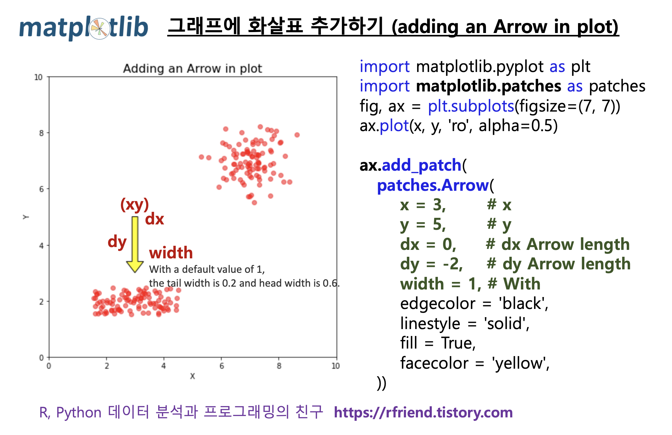
[ Reference ]
* Python matplotlib's Inheritance Diagrams
: https://matplotlib.org/stable/api/artist_api.html#artist-api
* Reference for matplotlib artists
* Python matplotlib's Rectangle patch
: https://matplotlib.org/stable/api/_as_gen/matplotlib.patches.Rectangle.html
* Python matplotlib's Circle patch
: https://matplotlib.org/stable/api/_as_gen/matplotlib.patches.Circle.html
* Python matplotlib's scale-free Ellipse
: https://matplotlib.org/stable/api/_as_gen/matplotlib.patches.Ellipse.html
* Python matploblib's Polygon patch
: https://matplotlib.org/stable/api/_as_gen/matplotlib.patches.Polygon.html
* Python matplotlib's Arrow patch
: https://matplotlib.org/stable/api/_as_gen/matplotlib.patches.Arrow.html
이번 포스팅이 많은 도움이 되었기를 바랍니다.
행복한 데이터 과학자 되세요! :-)

'Python 분석과 프로그래밍 > Python 그래프_시각화' 카테고리의 다른 글
| [Python] Plotly 를 이용해서 3차원 산점도와 표면도 그리기 (3D Scatter and Surface Plot in Python using Plotly) (0) | 2023.06.11 |
|---|---|
| [Python] 의사결정나무 시각화 (Visualization of Decision Tree using Python) (5) | 2022.08.22 |
| [Python matplotlib] 버블 그래프 (Bubble chart) (2) | 2022.02.01 |
| [Python] HoloViews 모듈을 사용해서 Sankey Diagram 그리기 (0) | 2022.01.23 |
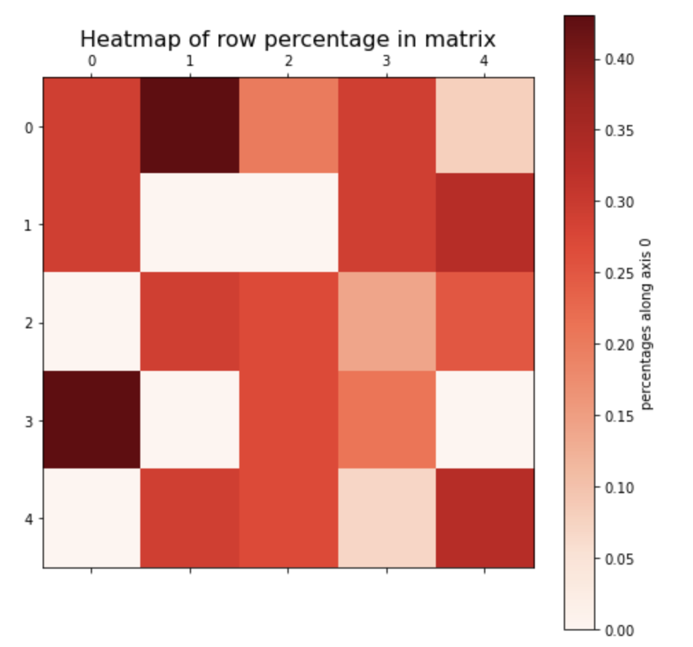
| [Python matplotlib] numpy 2D array의 행 기준, 열 기준 백분율을 구해서 히트맵 그리기 (0) | 2022.01.16 |