R, Python 분석과 프로그래밍의 친구 (by R Friend)

지난번 포스팅에서는 차원 축소란 무엇이고 왜 하는지(https://rfriend.tistory.com/736)와 투영(projection) 방법을 사용하는 주성분 분석(PCA)을 통한 차원 축소 (https://rfriend.tistory.com/751) 에 대해서 소개하였습니다. 

이번 포스팅에서는 manifold learning approche 에 해당하는 비지도학습, 비선형 차원축소 방법으로서 LLE (Locally Linear Embedding) 알고리즘을 설명하겠습니다. 

(1) 매니폴드 학습 (Manifold Learning)

(2) Locally Linear Embedding (LLE) 알고리즘

(3) sklearn 을 사용한 LLE 실습

(1) 매니폴드 학습 (Maniflod Learning)

먼저 매니폴드 학습(Manifold Learning)에 대해서 간략하게 살펴보고 넘어가겠습니다.

매니폴드란 각 점 근처의 유클리드 공간과 국부적으로 유사한 위상 공간을 말합니다. (A manifold is a topological space that locally resembles Eucludian space near each point.) [1]  d-차원의 매니폴드는 n-차원 공간 (이때 d < n) 의 부분으로서 d-차원의 초평면(d-dimensional hyperplane)을 국부적으로 닮았습니다. 아래의 3차원 공간의 Swiss Roll 에서 데이터의 구성 특성과 속성을 잘 간직한 2차원의 평면(plane)을 생각해볼 수 있는데요, Swiss Roll 을 마치 돌돌 말린 종이(매니폴드)를 펼쳐서 2차원 공간으로 표현해본 것이 오른쪽 그림입니다. 

매니폴드 학습(Manifold Learning)이란 데이터에 존재하는 매니폴드를 모델링하여 차원을 축소하는 기법을 말합니다. 매니폴드 학습은 대부분 실세계의 고차원 데이터가 훨씬 저차원의 매니폴드에 가깝게 놓여있다는 매니폴드 가정(Manifold Assumption) 혹은 매니폴드 가설(Maniflod Hypothesis)에 기반하고 있습니다. [2] 

위의 비선형인 3차원 Swiss Roll 데이터를 선형 투영 기반의 주성분 분석(PCA, Principal Component Analysis)이나 다차원척도법(MDS, Multi-Dimensional Scaling) 로 2차원으로 차원을 축소하려고 하면 데이터 내 존재하는 매너폴드를 학습하지 못하고 데이터가 뭉개지고 겹쳐지게 됩니다. 

매니폴드 가설은 분류나 회귀모형과 같은 지도학습을 할 때 고차원의 데이터를 저차원의 매니폴드 공간으로 재표현했을 때 더 간단하고 성과가 좋을 것이라는 묵시적인 또 다른 가설과 종종 같이 가기도 합니다. 하지만 이는 항상 그런 것은 아니며, 데이터셋이 어떻게 구성되어 있느냐에 전적으로 의존합니다. 

(2) Locally Linear Embedding (LLE) 알고리즘

LLE 알고리즘은 "Nonlinear Dimensionality Reduction by Locally Linear Embedding (2000)" [3] 논문에서 주요 내용을 간추려서 소개하겠습니다. 

LLE 알고리즘은 주성분분석이나(PCA) 다차원척도법(MDS)와는 달리 광범위하게 흩어져있는 데이터 점들 간의 쌍을 이룬 거리를 추정할 필요가 없습니다. LLE는 국소적인 선형 적합으로 부터 전역적인 비선형 구조를 복원합니다 (LLE revocers global nonlinear structure from locally linear fits.). 

논문에서 소개한 LLE 3단계 절차(steps of locally linear embedding)는 꽤 간단합니다. 

    (1단계) 각 데이터 점의 이웃을 선택 (Select neighbors)

    (2단계) 이웃으로부터 선형적으로 가장 잘 재구성하는 가중치를 계산 (Reconstruct with linear weights)

    (3단계) 가중치를 사용해 저차원의 임베딩 좌표로 매핑 (Map to embedded coordinates)

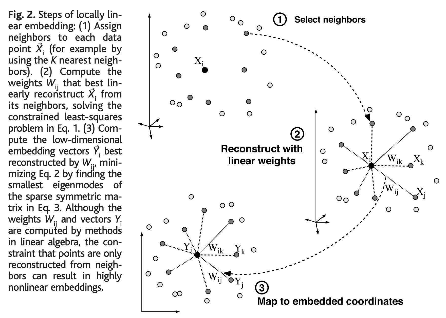
1단계에서 각 데이터 점별로 이웃을 할당할 때는 데이터 점들 간의 거리를 계산하는데요, 가령 K 최근접이웃(K nearest neighbors) 기법을 사용할 수 있습니다. 

2단계에서 각 데이터 점들의 이웃들로부터 각 점을 가장 잘 재구성하는 선형 회귀계수(linear coefficients, linear weights)를 계산해서 국소적인 기하 특성을 간직한 매너폴드를 학습합니다.  아래는 재구성 에러를 측정하는 비용함수인데요, 원래의 데이터점과 이웃들로 부터 계산한 선형 모형으로 재구성한 값과의 거리를 제곱하여 모두 더한 값입니다. 

위의 비용함수를 최소로 하는 가중치 벡터 Wij 를 계산하게 되는데요, 이때 2가지 제약조건(constraints)이 있습니다. 

  - (a) 각 데이터 점은 단지 그들의 이웃들로 부터만 재구성됩니다.

          (만약 Xj 가 Xi의 이웃에 속하지 않는 데이터점이면 가중치 Wij = 0 이 됩니다.)

  - (b) 가중치 행렬 행의 합은 1이 됩니다. (sum(Wij) = 1) 

위의 2가지 제약조건을 만족하면서 비용함수를 최소로 하는 가중치 Wij 를 구하면 특정 데이터 점에 대해 회전(rotations), 스케일 조정(recalings), 그리고 해당 데이터 점과 인접한 데이터 점의 변환(translations) 에 있어 대칭(symmetry)을 따릅니다. 이 대칭에 의해서 (특정 참조 틀에 의존하는 방법과는 달리) LLE의 재구성 가중치는 각 이웃 데이터들에 내재하는 고유한 기하학적 특성(저차원의 매너폴드)을 모델링할 수 있게됩니다. 

3단계에서는 고차원(D) 벡터의 각 데이터 점 Xi 를 위의 2단계에서 계산한 가중치를 사용하여 매니폴드 위에 전역적인 내부 좌표를 표현하는 저차원(d) 벡터 Yi 로 매핑합니다.  이것은 아래의 임베팅 비용 함수를 최소로 하는 저차원 좌표 Yi (d-mimensional coordinates) 를 선택하는 것으로 수행됩니다. 

임베팅 비용 함수는 이전의 선형 가중치 비용함수와 마찬가지로 국소 선형 재구성 오차를 기반으로 합니다. 하지만 여기서 우리는 Yi 좌표를 최적화하는 동안 선형 가중치 Wij 를 고정합니다. 임베팅 비용 함수는 희소 N x N 고유값 문제(a sparse N X N eignevalue problem)를 풀어서 최소화할 수 있습니다. 이 선형대수 문제를 풀면 하단의 d차원의 0이 아닌 고객벡터는 원점을 중심으로 정렬된 직교 좌표 집합을 제공합니다. 

LLE 알고리즘은 희소 행렬 알고리듬(sparse matrix algorithms)을 활용하기 위해 구현될 때 비선형 차원축소 기법 중 하나인 Isomap 보다 더 빠른 최적화와 많은 문제에 대해 더 나은 결과를 얻을 수 있는 몇 가지 장점이 있습니다. [4]

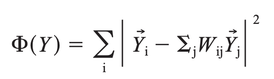
아래에 3차원 Swiss Roll 데이터를 여러가지 비선형 차원 축소 기법을 사용해서 적용한 결과인데요 [5], LLE 는 수행 시간이 짧은 장점이 있지만 매니폴드가 약간 찌그러져 있는 한계가 있는 반면에, Isomap과 Hessian LLE 는 국지적인 데이터 형상과 관계를 잘 재표현한 저차원 매니폴드를 잘 잡아내지만 수행 시간이 LLE 대비 굉장히 오래걸리는 단점이 있습니다. 

(3) sklearn 을 사용한 LLE 실습

먼저 sklearn 모듈의 make_swiss_roll 메소드를 사용해서 데이터 점 1,000개를 가지는 3차원의 Swiss Roll 샘플 데이터셋을 만들어보겠습니다. X 는 데이터 점이고, t는 매니폴드 내 점의 주 차원에 따른 샘플의 단변량 위치입니다. 

## Swiss Roll sample dataset
## ref: https://scikit-learn.org/stable/modules/generated/sklearn.datasets.make_swiss_roll.html
from sklearn.datasets import make_swiss_roll

X, t = make_swiss_roll(n_samples=1000, noise=0.1, random_state=1004)


## X: The points.
X[:5]
# array([[ 1.8743272 , 18.2196214 , -4.75535504],
#        [12.43382272, 13.9545544 ,  2.91609936],
#        [ 8.02375359, 14.23271056, -8.67338106],
#        [12.23095692,  2.37167446,  3.64973091],
#        [-8.44058318, 15.47560926, -5.46533069]])


## t: The univariate position of the sample according to the main dimension of the points in the manifold.
t[:10]
# array([ 5.07949952, 12.78467229, 11.74798863, 12.85471755,  9.99011767,
#         5.47092408,  6.89550966,  6.99567358, 10.51333994, 10.43425738])

다음으로 sklearn 모듈에 있는 LocallyLinearEmbedding 메소드를 사용해서 위에서 생성한 Swiss Roll 데이터에 대해 LLE 알고리즘을 적용하여 2차원 데이터로 변환을 해보겠습니다. 

## Manifold Learning
from sklearn.manifold import LocallyLinearEmbedding

lle = LocallyLinearEmbedding(n_components=2, n_neighbors=10)

X_reduced_lle = lle.fit_transform(X)

X_reduced_lle[:10]
# array([[-0.0442308 ,  0.0634603 ],
#        [ 0.04241534,  0.01060574],
#        [ 0.02712308,  0.01121903],
#        [ 0.04396569, -0.01883799],
#        [ 0.00275144,  0.01550906],
#        [-0.04178513,  0.05415933],
#        [-0.03073913,  0.023496  ],
#        [-0.02880368, -0.0230327 ],
#        [ 0.0109238 , -0.02566617],
#        [ 0.00979253, -0.02309815]])

마지막으로 matplotlib 모듈을 사용해서 2차원 평면에 위에서 LLE 로 매핑한 데이터를 시각화해보겠습니다. 색깔을 t 로 구분하였습니다. 

## 2D Scatter Plot
import matplotlib.pyplot as plt

plt.rcParams['figure.figsize'] = (8, 8)
plt.scatter(X_reduced_lle[:, 0], X_reduced_lle[:, 1], c=t, cmap=plt.cm.hot)
plt.title("Unrolled Swiss Roll by LLE", fontsize=20)
plt.xlabel("$y_1$", fontsize=14)
plt.ylabel("$y_2$", fontsize=14)
plt.axis([-0.065, 0.055, -0.1, 0.12])
plt.grid(True)

plt.show()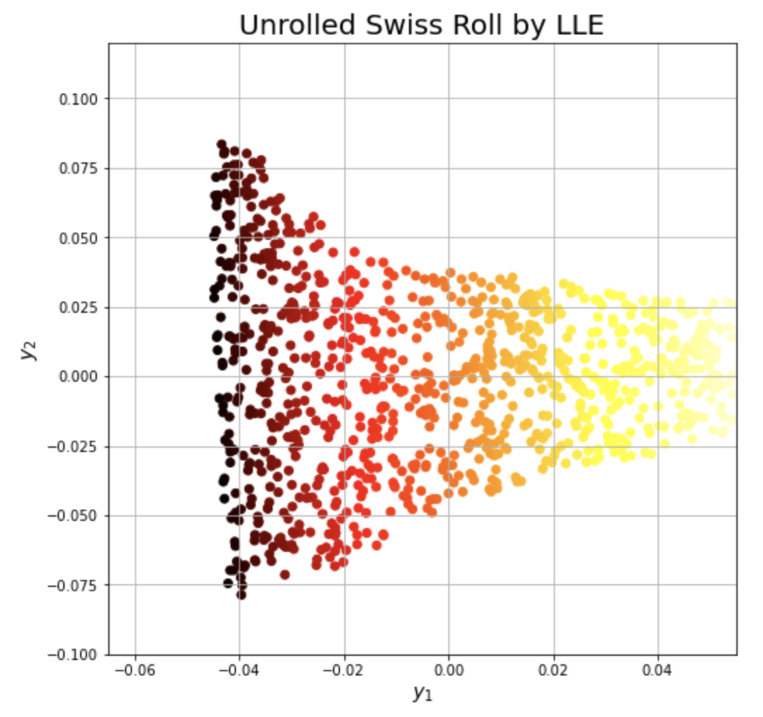

[Reference]

[1] Wikipedia, "Manifold", https://en.wikipedia.org/wiki/Manifold

[2] Aurelien Geron, "Hands-On Machine Learning with Scikit-Learn & Tensorflow"

[3] Sam T. Roweis, Lawrence K. Saul, "Nonlinear Dimensionality Reduction by Locally Linear Embedding"

[4] Wikipedia, "Nonlinear Dimensionality Reduction",  https://en.wikipedia.org/wiki/Nonlinear_dimensionality_reduction

[5] Nik Melchior, "Manifold Learning, Isomap and LLE":  https://www.cs.cmu.edu/~efros/courses/AP06/presentations/melchior_isomap_demo.pdf 

이번 포스팅이 많은 도움이 되었기를 바랍니다. 

행복한 데이터 과학자 되세요!  :-)

지난 포스팅에서는 차원 축소란 무엇이고 왜 하는지, 무슨 방법이 있는지에 대해서 알아보았습니다.

(https://rfriend.tistory.com/736)  차원축소하는 방법에는 크게 Projection-based dimensionality reduction, Manifold Learning 의 두가지 방법이 있다고 했습니다. 

이번 포스팅에서는 투사를 통한 차원축소 방법(dimensionality reduction via projection approach) 으로서 주성분분석을 통한 차원축소(dimensionality reduction using PCA, Principal Component Analysis)에 대해서 소개하겠습니다. 

(1) 주성분분석(PCA, Principal Component Analysis)을 통한 차원 축소

(2) 특이값 분해 (SVD, Singular Value Decomposition)을 통한 차원 축소

(1) 주성분 분석(PCA, Principal Component Analysis)을 통한 차원 축소

주성분 분석(PCA)의 핵심 아이디어만 간략하게 소개하자면요, 피쳐 공간(Feature Space)에서 데이터의 분산을 최대로 잡아낼 수 있는 축을 제1 주성분 축으로 잡고, 이 제1 주성분 축과 직교(orthogonal)하는 축을 제2 주성분 축으로 잡고, ..., 이렇게 최대 변수의 개수 p 개 만큼 주성분 축을 잡아줍니다. (물론, 차원축소를 하는 목적이면 주성분 개수 m 이 변수 개수 p 보다는 작아야 겠지요). 그리고 축을 회전시켜주면 돼요. 

아래의 예시 도면을 보면 파란색 제 1 주성분 축 (1st principal component axis)이 데이터 분산을 가장 많이 설명하고 있는 것을 알 수 있습니다. 빨간색 점선의 제 2 주성분 축(2nd principal component axis) 은 제1 주성분 축과 직교하구요. 

이제 Python 을 가지고 실습을 해볼께요. 

(R로 주성분 분석 하는 것은 https://rfriend.tistory.com/61 를 참고하세요.)

먼저 예제로 사용할 iris 데이터셋을 가져오겠습니다. sepal_length, sepal_width, petal_length, petal_width 의 4개 변수를 가진 데이터셋인데요, 4개 변수 간 상관관계 분석을 해보니 상관계수가 0.8 이상으로 꽤 높게 나온 게 있네요. 주성분분석으로 차원축소 해보면 이쁘게 나올거 같아요. 

import numpy as np
import pandas as pd
import matplotlib.pyplot as plt

## loading IRIS dataset
from sklearn.datasets import load_iris
data = load_iris()


data['data'][:10]
# array([[5.1, 3.5, 1.4, 0.2],
#        [4.9, 3. , 1.4, 0.2],
#        [4.7, 3.2, 1.3, 0.2],
#        [4.6, 3.1, 1.5, 0.2],
#        [5. , 3.6, 1.4, 0.2],
#        [5.4, 3.9, 1.7, 0.4],
#        [4.6, 3.4, 1.4, 0.3],
#        [5. , 3.4, 1.5, 0.2],
#        [4.4, 2.9, 1.4, 0.2],
#        [4.9, 3.1, 1.5, 0.1]])


## converting into pandas DataFrame
iris_df = pd.DataFrame(
    data['data'], 
    columns=['sepal_length', 'sepal_width', 
             'petal_length', 'petal_width'])

iris_df.head()
# 	sepal_length	sepal_width	petal_length	petal_width
# 0	5.1	3.5	1.4	0.2
# 1	4.9	3.0	1.4	0.2
# 2	4.7	3.2	1.3	0.2
# 3	4.6	3.1	1.5	0.2
# 4	5.0	3.6	1.4	0.2


## correlation matrix
iris_df.corr()
# 	sepal_length	sepal_width	petal_length	petal_width
# sepal_length	1.000000	-0.117570	0.871754	0.817941
# sepal_width	-0.117570	1.000000	-0.428440	-0.366126
# petal_length	0.871754	-0.428440	1.000000	0.962865
# petal_width	0.817941	-0.366126	0.962865	1.000000

주성분 분석은 비지도 학습 (Unsupervised Learning) 이다보니 정답이라는게 없습니다. 그래서 분석가가 주성분의 개수를 지정해주어야 하는데요, 주성분의 개수가 적을 수록 차원 축소가 많이 되는 반면 정보 손실(information loss)가 발생하게 되며, 반면 주성분 개수가 많을 수록 정보 손실은 적겠지만 차원 축소하는 의미가 퇴색됩니다. 그래서 적절한 주성분 개수를 선택(hot to decide the number of principal components)하는게 중요한데요, 주성분의 개수별로 설명 가능한 분산의 비율 (percentage of explained variance by principal components) 을 많이 사용합니다. 

아래의 예에서는 첫번째 주성분이 분산의 92.4%를 설명하고, 두번째 주성분이 분산의 5.3%를 설명하므로, 주성분 1 & 2 까지 사용하면 전체 분산의 97.7%를 설명할 수 있게 됩니다. (즉, 원래 4개 변수를 2개의 차원으로 축소하더라도 분산의 97.7%를 설명 가능하다는 뜻) 

참고로, 만약 주성분분석 결과를 지도학습(가령, 회귀분석)의 설명변수 인풋으로 사용한다면, cross validation을 사용해서 주성분 개수별로 모델의 성능을 평가(가령, 회귀분석의 경우 MSE)해서, 모델 성능지표가 가장 좋은 주성분 개수를 선택하는 것도 좋은 방법입니다. 

## how to decide the number of Principal Components
from sklearn.decomposition import PCA

pca = PCA(random_state=1004)
pca.fit_transform(iris_df)


## percentage of variance explained
print(pca.explained_variance_ratio_)
# [0.92461872 0.05306648 0.01710261 0.00521218]


## Principal 1 & 2 explain about 97.8% of variance
plt.rcParams['figure.figsize'] = (7, 7)
plt.plot(range(1, iris_df.shape[1]+1), pca.explained_variance_ratio_)
plt.xlabel("number of Principal Components", fontsize=12)
plt.ylabel("% of Variance Explained", fontsize=12)
plt.show()

이제 주성분 개수를 2개로 지정(n_components=2)해서 주성분 분석을 실행해보겠습니다. Python의 sklearn 모듈의 decomposition.PCA 메소드를 사용하겠습니다. 

## Dimensionality Reduction with n_components=2
pca = PCA(n_components=2, random_state=1004)
iris_pca = pca.fit_transform(iris_df)


iris_pca[:10]
# array([[-2.68412563,  0.31939725],
#        [-2.71414169, -0.17700123],
#        [-2.88899057, -0.14494943],
#        [-2.74534286, -0.31829898],
#        [-2.72871654,  0.32675451],
#        [-2.28085963,  0.74133045],
#        [-2.82053775, -0.08946138],
#        [-2.62614497,  0.16338496],
#        [-2.88638273, -0.57831175],
#        [-2.6727558 , -0.11377425]])

위에서 실행한 주성분분석 결과를 가지고 시각화를 해보겠습니다. 4개 변수를 2개의 차원으로 축소를 했기 때문에 2차원의 산점도로 시각화를 할 수 있습니다. 이때 iris 데이터셋의 target 속성정보를 이용해서 붓꽃의 품종별로 색깔과 모양을 달리해서 산점도로 시각화해보겠습니다. 

## Visualization

## target
data['target'][:5]
# array([0, 0, 0, 0, 0])


## mapping target name using numpy vectorization
species_map_dict = {
    0: 'setosa', 
    1: 'versicolor', 
    2: 'virginica'
}

iris_pca_df = pd.DataFrame({
    'pc_1': iris_pca[:, 0], 
    'pc_2': iris_pca[:, 1], 
    'species': np.vectorize(species_map_dict.get)(data['target']) # numpy broadcasting
})


iris_pca_df.head()
# pc_1	pc_2	species
# 0	-2.684126	0.319397	setosa
# 1	-2.714142	-0.177001	setosa
# 2	-2.888991	-0.144949	setosa
# 3	-2.745343	-0.318299	setosa
# 4	-2.728717	0.326755	setosa


import seaborn as sns
import matplotlib.pyplot as plt

plt.rcParams['figure.figsize'] = (7, 7)
sns.scatterplot(
    x='pc_1', 
    y='pc_2',
    hue='species', 
    style='species',
    s=100,
    data=iris_pca_df
)

plt.title('PCA result of IRIS dataset')
plt.xlabel('Principal Component 1', fontsize=14)
plt.ylabel('Principal Component 2', fontsize=14)
plt.show()

(2) 특이값 분해 (SVD, Singular Value Decomposition)을 통한 차원 축소

선형대수의 특이값 분해의 결과로 나오는 U, sigma, V 에서 V 가 주성분 분석의 주성분에 해당합니다.  

특이값 분해(SVD, Singular Value Decomposition)에 대한 이론적인 소개는 https://rfriend.tistory.com/185 를 참고하세요. 

numpy 모듈의 linalg.svd 메소드를 사용하여 특이값 분해를 하려고 할 때 먼저 데이터 표준화(standardization)을 수작업으로 진행해 줍니다. (sklearn 으로 주성분분석을 할 때 sklearn 모듈이 내부적으로 알아서 표준화해서 진행해줌). 

## Standardization first
from sklearn.preprocessing import StandardScaler

scaler = StandardScaler()
X_scaled = scaler.fit_transform(data['data'])


## PCA assumes that the dataset is centered around the origin.
X_centered = data['data'] - data['data'].mean(axis=0)
X_centered[:5]
# array([[-0.74333333,  0.44266667, -2.358     , -0.99933333],
#        [-0.94333333, -0.05733333, -2.358     , -0.99933333],
#        [-1.14333333,  0.14266667, -2.458     , -0.99933333],
#        [-1.24333333,  0.04266667, -2.258     , -0.99933333],
#        [-0.84333333,  0.54266667, -2.358     , -0.99933333]])

웨에서 표준화한 데이터를 numpy 모듈의 linalg.svd 메소드를 사용하여 특이값 분해를 해준 후에, V 를 transpose (T) 해주어서 첫번째와 두번째 열의 값을 가져오면 제1 주성분, 제2 주성분을 얻을 수 있습니다. 

## standard matrix factorization using SVD
U, s, V = np.linalg.svd(X_scaled.T)


## V contains all the principal components
pc_1 = V.T[:, 0]
pc_2 = V.T[:, 1]


## check pc_1, pc_2
pc_1[:10]
# array([0.10823953, 0.09945776, 0.1129963 , 0.1098971 , 0.11422046,
#        0.099203  , 0.11681027, 0.10671702, 0.11158214, 0.10439809])


pc_2[:10]
# array([-0.0409958 ,  0.05757315,  0.02920003,  0.05101939, -0.0552418 ,
#        -0.12718049, -0.00406897, -0.01905755,  0.09525253,  0.04005525])

위에서 특이값분해(SVD)로 구한 제1 주성분, 제2 주성분을 가지고 산점도를 그려보겠습니다. 이때 iris 의 target 별로 색깔과 모양을 달리해서 시각화를 해보겠습니다. 

## Visualization

iris_svd_df = pd.DataFrame({
    'pc_1': pc_1, 
    'pc_2': pc_2, 
    'species': np.vectorize(species_map_dict.get)(data['target']) # numpy broadcasting
})


import seaborn as sns
import matplotlib.pyplot as plt

plt.rcParams['figure.figsize'] = (7, 7)
sns.scatterplot(
    x='pc_1', 
    y='pc_2',
    hue='species', 
    style='species',
    s=100,
    data=iris_svd_df
)

plt.title('SVD result of IRIS dataset')
plt.xlabel('Principal Component 1', fontsize=14)
plt.ylabel('Principal Component 2', fontsize=14)
plt.show()

이번 포스팅이 많은 도움이 되었기를 바랍니다. 

행복한 데이터 과학자 되세요. 

이번 포스팅에서는 Python 을 이용해서 의사결정나무 (Decision Tree) 를 시각화하는 3가지 방법을 소개하겠습니다. 

(1) sklearn.tree.export_text 메소드를 이용해서 의사결정나무를 텍스트로 인쇄하기 (text representation)

(2) sklearn.tree.plot_tree 메소드와 matplotlib 을 이용해서 의사결정나무 시각화

(3) sklearn.tree.export_graphviz 메소드와 graphviz 를 이용해서 의사결정나무 시각화

먼저, 예제로 사용할 iris 데이터셋과 필요한 모듈을 불어오겠습니다. 

import numpy as np
import pandas as pd
import matplotlib.pyplot as plt 

df = pd.DataFrame({
    'x1': [1, 2, 2, 2, 2, 3, 3, 4, 5, 5], 
    'x2': [2, 2, 3, 4, 5, 4, 6, 3, 2, 5], 
    'cat': [0, 1, 1, 0, 0, 1, 0, 1, 1, 0]
})


df

# x1	x2	cat
# 0	1	2	0
# 1	2	2	1
# 2	2	3	1
# 3	2	4	0
# 4	2	5	0
# 5	3	4	1
# 6	3	6	0
# 7	4	3	1
# 8	5	2	1
# 9	5	5	0


## scatter plot
import seaborn as sns

plt.figure(figsize=(7, 7))
sns.scatterplot(x='x1', y='x2', hue='cat', style='cat', s=100, data=df)
plt.show()

(0) sklearn.tree 메소드를 이용해서 의사결정나무(Decision Tree) 모델 훈련하기

from sklearn.tree import DecisionTreeClassifier
from sklearn.model_selection import cross_val_score
from sklearn import tree

## getting X, y values
X = df[['x1', 'x2']]
y = df['cat']

## initiating DecisionTreeClassifer method
dt_clf = DecisionTreeClassifier(random_state = 1004)


## fitting a decision tree classifier
dt_clf_model = dt_clf.fit(X, y)


## feature importances
dt_clf_model.feature_importances_

#array([0.43809524, 0.56190476])

(1) sklearn.tree.export_text 메소드를 이용해서 의사결정나무를 텍스트로 인쇄하기 (text representation)

의사결정나무 모델을 적합한 후에 사용자 인터페이스가 없는 애플리케이션에서 로그(log) 텍스트로 모델 적합 결과를 확인할 때 사용할 수 있습니다. 또는 의사결정나무의 적합된 룰을 SQL 로 구현하여 운영 모드로 적용하고자 할 때 아래처럼 텍스트로 인쇄를 하면 유용하게 사용할 수 있습니다. 

## Text Representation
dt_clf_model_text = tree.export_text(dt_clf_model)

print(dt_clf_model_text)

|--- feature_1 <= 4.50
|   |--- feature_0 <= 1.50
|   |   |--- class: 0
|   |--- feature_0 >  1.50
|   |   |--- feature_1 <= 3.50
|   |   |   |--- class: 1
|   |   |--- feature_1 >  3.50
|   |   |   |--- feature_0 <= 2.50
|   |   |   |   |--- class: 0
|   |   |   |--- feature_0 >  2.50
|   |   |   |   |--- class: 1
|--- feature_1 >  4.50
|   |--- class: 0

(2) sklearn.tree.plot_tree 메소드와 matplotlib 을 이용해서 의사결정나무 시각화

(3)번 처럼 Graphviz 를 설치하지 않아도, matplotlib 을 사용해서 간편하게 의사결정나무를 시각화 할 때 유용합니다. 편리한 대신에 (3)번 Graphviz 대비 자유도가 떨어지는 단점이 있습니다. 

## Plot Tree with plot_tree
fig = plt.figure(figsize=(15, 8))
_ = tree.plot_tree(dt_clf_model, 
                  feature_names=['x1', 'x2'],
                  class_names=['0', '1'],
                  filled=True)

(3) sklearn.tree.export_graphviz 메소드와 graphviz 를 이용해서 의사결정나무 시각화

Graphviz 의 시각화 기능을 fully 사용할 수 있으므로 매우 강력한 시각화 방법이라고 할 수 있습니다. 

Graphviz 설치하고 Decision Tree 시각화하기는 https://rfriend.tistory.com/382 를 참고하세요. 

DOT language 에 대해서는 https://graphviz.org/doc/info/lang.html 를 참고하세요. 

## Visualizing Tree using Graphviz
from sklearn import tree
import graphviz

## exporting tree in DOT format
## refer to: https://scikit-learn.org/stable/modules/generated/sklearn.tree.export_graphviz.html
tree_dot = tree.export_graphviz(
    dt_clf_model, 
    feature_names=['x1', 'x2'], 
    class_names=['0', '1'],
    filled=True
)


## draw graph using Graphviz
dt_graph = graphviz.Source(tree_dot, format='png')
dt_graph

이번 포스팅이 많은 도움이 되었기를 바랍니다. 

행복한 데이터 과학자 되세요~!

이번 포스팅에서는 Python을 사용해서 

(1) 텍스트 데이터 전처리 (text data pre-processing)

(2) 토큰화 (tokenization)

하는 방법을 소개하겠습니다. 

(1) 텍스트 데이터 전처리 (text data pre-processing)

텍스트 데이터 전처리를 하는데는 (a) Python의 텍스트 처리 내장 메소드 (Python built-in methods)와 (b) 정규 표현식 매칭 연산(regular expression matching operations)을 제공하는 Python re 패키지를 사용하겠습니다. re 패키지는 Python을 설치할 때 디폴트로 같이 설치가 되므로 별도로 설치할 필요는 없습니다. 

예제로 사용할 Input 텍스트는 인터넷쇼핑몰의 고객별 거래내역에 있는 구매 품목 텍스트 데이터이며, Output 은 텍스트 전처리 후의 고객별 구매 품목의 리스트입니다. 

예) Input: '**[세일]** 말티즈 강아지사료 습식 소프트 신 3종 15Kg 39,000원!!...외5건'

예) Output: [말티즈, 강아지사료, 습식, 소프트]

[ 텍스트 데이터 전처리 절차 ]

    (1-1) [], (), {}, <> 괄호와 괄호 안 문자 제거하기

    (1-2) '...외', '...총' 제거하기

    (1-3) 특수문자, 숫자 제거

    (1-4) 단위 제거: cm, km, etc.

    (1-5) 공백 기준으로 분할하기

    (1-6) 글자 1개만 있으면 제외하기

    (1-7) 텍스트 데이터 전처리 사용자 정의함수(User Defined Function) 정의 

    (1-8) pandas DataFrame의 텍스트 칼럼에 데이터 전처리 사용자 정의함수 적용

(1-1) [], (), {}, <> 괄호와 괄호 안 문자 제거하기

Python의 정규 표현식(regular expression)을 다루는 re 패키지를 사용해서 다양한 형태의 괄호와 괄호안의 문자를 매칭한 후에 '' 로 대체함으로써 결과적으로 제거하였습니다. re.sub() 는 pattern 과 매치되는 문자열을 repl 의 문자열로 대체를 시켜줍니다. 

정규표현식에서 문자 클래스를 만드는 메타 문자인 [ ] 로 만들어지는 정규표현식은 [ ]사이에 들어가는 문자 중 어느 한개라도 매치가 되면 매치를 시켜줍니다. 가령, [abc] 의 경우 'a', 'b', 'c' 중에서 어느 하나의 문자라도 매치가 되면 매치가 되는 것으로 간주합니다. 

## Python Regular expression operations
import re

## sample text
s = '**[세일]** 말티즈 강아지사료 습식 소프트 신 3종 15Kg 39,000원!!...외5건'


## (1-1) [], (), {}, <> 괄호와 괄호 안 문자 제거하기
pattern = r'\([^)]*\)'  # ()
s = re.sub(pattern=pattern, repl='', string=s)

pattern = r'\[[^)]*\]'  # []
s = re.sub(pattern=pattern, repl='', string=s)

pattern = r'\<[^)]*\>'  # <>
s = re.sub(pattern=pattern, repl='', string=s)

pattern = r'\{[^)]*\}'  # {}
s = re.sub(pattern=pattern, repl='', string=s)

print(s)
[Out] 
# **** 말티즈 강아지사료 습식 소프트 신 3종 15Kg 39,000원!!...외5건

(1-2) '...외', '...총' 제거하기

Python의 내장 문자열 메소드인 replace() 를 사용해서 '...외', '...총' 을 ' ' 로 대체함으로써 제거하였습니다. 

## (1-2) '...외', '...총' 제거하기
s = s.replace('...외', ' ')
s = s.replace('...총', ' ')

print(s)
[Out]
# **** 말티즈 강아지사료 습식 소프트 신 3종 15Kg 39,000원!! 5건

(1-3) 특수문자, 숫자 제거

정규표현식에서 하이픈(-)은 from ~ to 의 범위를 나타냅니다. [a-zA-Z] 는 소문자와 대문자 영어 모두를 의미하며, [가-힣] 은 한글 전체를 의미합니다. 

정규표현식에서 [^] 는 not 의 의미이며, 아래의 [^a-zA-Z가-힣] 은 앞에 '^' 가 붙었으므로 영어와 한글이 아닌(not, ^) 문자, 즉 특수문자와 숫자와 매칭이 됩니다. 

## (1-3) 특수문자, 숫자 제거
pattern = r'[^a-zA-Z가-힣]'
s = re.sub(pattern=pattern, repl=' ', string=s)

print(s)
[Out] 
# 말티즈 강아지사료 습식 소프트 신  종   Kg       원    건

(1-4) 단위 제거: cm, km, etc.

## (1-4) 단위 제거: cm, km, etc.
units = ['mm', 'cm', 'km', 'ml', 'kg', 'g']
for unit in units:
    s = s.lower() # 대문자를 소문자로 변환
    s = s.replace(unit, '')
    
print(s)
[Out] 
# 말티즈 강아지사료 습식 소프트 신  종          원    건

(1-5) 공백 기준으로 분할하기

Python 내장형 문자열 메소드인 split() 을 사용해서 공백(space)을 기준으로 문자열을 분할하였습니다. 

## (1-5) 공백 기준으로 분할하기
s_split = s.split()

print(s_split)
[Out] 
# ['말티즈', '강아지사료', '습식', '소프트', '신', '종', '원', '건']

(1-6) 글자 1개만 있으면 제외하기

글자 길이가 1 보다 큰 (len(word) != 1) 글자만 s_list 의 리스트에 계속 추가(append) 하였습니다. 

## (1-6) 글자 1개만 있으면 제외하기
s_list = []
for word in s_split:
    if len(word) !=1:
        s_list.append(word)
        
print(s_list)
[Out] 
# ['말티즈', '강아지사료', '습식', '소프트']

(1-7) 텍스트 데이터 전처리 사용자 정의함수(User Defined Function) 정의 

위의 (1-1) ~ (1-6) 까지의 텍스트 전처리 과정을 아래에 사용자 정의함수로 정의하였습니다. 문자열 s 를 input으로 받아서 텍스트 전처리 후에 s_list 의 단어들을 분할해서 모아놓은 리스트를 반환합니다. 

## 텍스트 전처리 사용자 정의함수(UDF of text pre-processing)
def text_preprocessor(s):
    import re
    
    ## (1) [], (), {}, <> 괄호와 괄호 안 문자 제거하기
    pattern = r'\([^)]*\)'  # ()
    s = re.sub(pattern=pattern, repl='', string=s)
    
    pattern = r'\[[^)]*\]'  # []
    s = re.sub(pattern=pattern, repl='', string=s)
    
    pattern = r'\<[^)]*\>'  # <>
    s = re.sub(pattern=pattern, repl='', string=s)
    
    pattern = r'\{[^)]*\}'  # {}
    s = re.sub(pattern=pattern, repl='', string=s)
    
    ## (2) '...외', '...총' 제거하기
    s = s.replace('...외', ' ')
    s = s.replace('...총', ' ')
    
    ## (3) 특수문자 제거
    pattern = r'[^a-zA-Z가-힣]'
    s = re.sub(pattern=pattern, repl=' ', string=s)
    
    ## (4) 단위 제거: cm, km, etc.
    units = ['mm', 'cm', 'km', 'ml', 'kg', 'g']
    for unit in units:
        s = s.lower() # 대문자를 소문자로 변환
        s = s.replace(unit, '')
        
    # (5) 공백 기준으로 분할하기
    s_split = s.split()
    
    # (6) 글자 1개만 있으면 제외하기
    s_list = []
    for word in s_split:
        if len(word) !=1:
            s_list.append(word)
            
    return s_list
    

## sample text
s = '**[세일]** 말티즈 강아지사료 습식 소프트 신 3종 15Kg 39,000원!!...외5건'

## apply the UDF above
s_list = text_preprocessor(s)
print(s_list)
[Out] 
# ['말티즈', '강아지사료', '습식', '소프트']

(1-8) pandas DataFrame의 텍스트 칼럼에 데이터 전처리 사용자정의함수 적용

pandas DataFrame에 위의 (1-7) 텍스트 전처리 사용자 정의함수를 적용하기 위해서는 apply() 와 lambda function 을 사용합니다. 

## pandas DataFrame
import pandas as pd

s1 = '**[세일] 몰티즈 강아지사료 습식 소프트 신 3종 15Kg 39,000원!!...외5건'
s2 = '[시크루즈] 50%+추가20%/여름신상 루즈핏 롱원피스/상하세트/점프슈트...외3건'
s3 = '올챌린지 KF94 마스크 100매 국내생산 여름용 황사 화이트...총2건'
s4 = '[최대혜택가] ##하림 용가리치킨 300gX3봉 외 닭가슴살/튀김 골라담기...외12건'
s5 = '[20%+15%] 종아리알 타파! 무로 요가링/마사지릴/압박스타킹/마사지볼...외4종'

df = pd.DataFrame({
    'id': [1, 2, 3, 4, 5], 
    'items': [s1, s2, s3, s4, s5]
})

print(df)
[Out]
#    id                                              items
# 0   1  **[세일] 몰티즈 강아지사료 습식 소프트 신 3종 15Kg 39,000원!!...외5건
# 1   2     [시크루즈] 50%+추가20%/여름신상 루즈핏 롱원피스/상하세트/점프슈트...외3건
# 2   3           올챌린지 KF94 마스크 100매 국내생산 여름용 황사 화이트...총2건
# 3   4   [최대혜택가] ##하림 용가리치킨 300gX3봉 외 닭가슴살/튀김 골라담기...외12건
# 4   5    [20%+15%] 종아리알 타파! 무로 요가링/마사지릴/압박스타킹/마사지볼...외4종


## Apply the text preprocessing UDF using apply() and lambda function
df['items_list'] = df['items'].apply(lambda s: text_preprocessor(s))


print(df['items'])
print('-------------'*5)
print(df['items_list'])
[Out]
# 0    **[세일] 몰티즈 강아지사료 습식 소프트 신 3종 15Kg 39,000원!!...외5건
# 1       [시크루즈] 50%+추가20%/여름신상 루즈핏 롱원피스/상하세트/점프슈트...외3건
# 2             올챌린지 KF94 마스크 100매 국내생산 여름용 황사 화이트...총2건
# 3     [최대혜택가] ##하림 용가리치킨 300gX3봉 외 닭가슴살/튀김 골라담기...외12건
# 4      [20%+15%] 종아리알 타파! 무로 요가링/마사지릴/압박스타킹/마사지볼...외4종
# Name: items, dtype: object
# -----------------------------------------------------------------
# 0                     [몰티즈, 강아지사료, 습식, 소프트]
# 1         [추가, 여름신상, 루즈핏, 롱원피스, 상하세트, 점프슈트]
# 2       [올챌린지, kf, 마스크, 국내생산, 여름용, 황사, 화이트]
# 3               [하림, 용가리치킨, 닭가슴살, 튀김, 골라담기]
# 4    [종아리알, 타파, 무로, 요가링, 마사지릴, 압박스타킹, 마사지볼]
# Name: items_list, dtype: object

위에 Jupyter Notebook 에서 pandas DataFrame을 출력한 결과가 중앙 정렬로 되어있어서 보기가 불편한데요, 아래처럼 좌측 정렬 (left alignment) 을 해서 보기에 편하도록 해보았습니다. 

## align text of pandas DataFrame to left in Jupyter Notebook
dfStyler = df.style.set_properties(**{'text-align': 'left'})
dfStyler.set_table_styles([dict(selector='th', props=[('text-align', 'left')])])

(2) 토큰화 (tokenization)

토큰화(Tokenization)는 말뭉치(Corpus)를 토큰이라고 불리는 단어 또는 문장으로 나누는 것을 말합니다. 이러한 토큰은 문맥(Context)을 이해하거나 NLP에 대한 모델을 개발하는 데 사용됩니다. 

POS 태킹 (Part-of-Speech Tagging) 은 널리 사용되는 자연어 처리 프로세스로, 단어의 정의와 문맥에 따라 언어의 특정 부분에 대응하여 텍스트(corpus)의 단어를 분류하는 것을 말합니다.

아래 코드는 위 (1)번의 텍스트 전처리에 이어서, 띄어쓰기가 제대로 되지 않아서 붙어 있는 단어들을, Python KoNLpy 패키지를 사용해서 형태소 분석의 명사를 기준으로 단어 토근화를 한 것입니다. ((2)번 words_tokonizer() UDF 안에 (1)번 text_preprocessor() UDF가 포함되어 있으며, 순차적으로 수행됩니다.)

KoNLpy 패키지는 Python으로 한국어 자연어 처리(NLP) 을 할 수 있게 해주는 패키지입니다. 그리고 Kkma 는 서울대학교의 IDS 랩에서 JAVA로 개발한 형태소 분석기(morphological analyzer)입니다.  

## insatll konlpy if it is not istalled yet
# ! pip install konlpy


## KoNLpy : NLP of the Korean language
## reference ==> https://konlpy.org/en/latest/
## Kkma is a morphological analyzer 
## and natural language processing system written in Java, 
## developed by the Intelligent Data Systems (IDS) Laboratory at SNU.
from konlpy.tag import Kkma


## define words tokenizer UDF
def words_tokonizer(text):
    from konlpy.tag import Kkma # NLP of the Korean language
    kkma = Kkma()
    
    words = []
    
    # Text preprocessing using the UDF above
    s_list = text_preprocessor(text)
    
    # POS tagging
    for s in s_list:
        words_ = kkma.pos(s)   
        
        # NNG indexing
        for word in words_:
            if word[1] == 'NNG':
                words.append(word[0])
            
    return words
    
    
## apply the UDF above as an example
words_tokonizer('강아지사료')
[Out] ['강아지', '사료']


words_tokonizer('상하세트')
[Out] ['상하', '세트']

위의 (2) words_tokenizer() UDF를 pandas DataFrame에 적용하기 위해서 apply() 함수와 lambda function 을 사용하면 됩니다. 

## apply the text tokenization UDF to pandas DataFrame using apply() and lambda function
df['items'].apply(lambda text: words_tokonizer(text))

[Out]
# 0 [몰티즈, 강아지, 사료, 습식, 소프트]
# 1 [추가, 여름, 신상, 루즈, 핏, 원피스, 상하, 세트, 점프, 슈트]
# 2 [챌린지, 마스크, 국내, 생산, 여름, 황사, 화이트]
# 3 [하림, 용가리, 치킨, 닭, 가슴살, 튀김]
# 4 [종아리, 타파, 무로, 요가, 링, 마사지, 압박, 스타, 킹, 마사지]
# Name: items, dtype: object

이번 포스팅이 많은 도움이 되었기를 바랍니다. 

행복한 데이터 과학자 되세요! :-)

이번 포스팅에서는 Python pandas의 문자열 Series에서 문자열 패턴 매칭을 통해서 특정 패턴이 포함되어 있는지 여부를 확인하고, 특정 매칭을 포함한 데이터를 가져오는 방법을 소개하겠습니다. 

(1) pandas 문자열 Series에서 한개의 문자열 패턴 매칭하기 
     : Series.str.contains(pattern)

(2) pandas DataFrame에서 한개의 문자열 패턴 매칭이 되는 데이터 가져오기

(3) pandas DataFrame에서 여러개의 문자열 패턴 매팅이 되는 데이터 가져오기

먼저, 예제로 사용할 문자열이 포함된 DataFrame을 만들어보겠습니다. pandas 의 contains() 함수를 사용해서 문자열 뿐만 아니라 NaN 값과 '1004' 숫자도 포함시켜서 문자열 매칭 시 처리방법을 소개하겠습니다. 

## importing modules
import numpy as np
import pandas as pd

## creating a pandas DataFrame with strings, NaN, digit
df = pd.DataFrame({
    'id': [1, 2, 3, 4, 5, 6, 7]
    , 'fruit': ['apple', 'PERSIMON', 'grapes', 'mango', 'peach and perl', 
                np.NaN, 
                '1004']
})


print(df)
#    id           fruit
# 0   1           apple
# 1   2        PERSIMON
# 2   3          grapes
# 3   4           mango
# 4   5  peach and perl
# 5   6             NaN
# 6   7            1004

(1) pandas 문자열 Series에서 한개의 문자열 패턴 매칭하기: Series.str.contains(pattern)

먼저, 위에서 만든 DataFrame에서 'fruit' 칼럼만 가져와서 's1' 이라는 이름의 Series 를 만들어보겠습니다. 

## pandas Series
s1 = df['fruit']

print(type(s1)) # padnas.Series
print(s1)

# <class 'pandas.core.series.Series'>
# 0             apple
# 1          PERSIMON
# 2            grapes
# 3             mango
# 4    peach and perl
# 5               NaN
# 6              1004
# Name: fruit, dtype: object

pandas 의 contains() 메소드는 '문자열 Series (Series of a string)' 을 대상으로 문자열 매칭을 해서 Boolean Series 를 반환합니다. contains() 메소드의 구문은 아래와 같습니다. 

Series.str.contains(pattern, case=True, flags=0, na=None, regex=True)

이때 Series.str.contains() 메소드는 문자열 Series에 대하여 패턴 매칭(pattern matching)을 할 때 문자열 그 자체(literal itself)와 함께 정규표현식(regex=True: regular expression)까지도 사용해서 패턴 매칭을 할 수 있으며, '대/소문자 구분 (case=True: case sensitive)하며, 'NaN' 값에 대해서는 'NaN'을 반환(na=None)합니다. 

아래 예에서는 문자열 Series 's1'에 대해서 문자열 'pe'가 들어있는 패턴 매칭을 해서 Boolean Series 를 반환한 예입니다. (대소문자 구분, NaN은  NaN 반환) 

## returning a Series of Booleans using a literal pattern
s1.str.contains('pe')

# 0    False
# 1    False   # <-- case sensitive
# 2     True
# 3    False
# 4     True
# 5      NaN   # <-- returning NaN for NaN values
# 6    False
# Name: fruit, dtype: object

(2) pandas DataFrame에서 한개의 문자열 패턴 매칭이 되는 데이터 가져오기

pandas DataFrame에서 특정 문자열 칼럼에 대해서 문자열 패턴 매칭한 결과인 Boolean Series 를 이용해서 해당 행의 값만 가져올 수 있습니다. 이때 만약 문자열 패턴 매칭 결과 Boolean Seires 에 NaN 값이 포함되어 있을 경우 아래와 같은 ValueError 가 발생합니다. 

ValueError: Cannot mask with non-boolean array containing NA / NaN valu

 ## ValueError: Cannot mask with non-boolean array containing NA / NaN values
df[df['fruit'].str.contains('pe')]

---------------------------------------------------------------------------
ValueError                                Traceback (most recent call last)
<ipython-input-5-ee5e3bc73f2f> in <module>
      1 ## ValueError: Cannot mask with non-boolean array containing NA / NaN values
----> 2 df[s1.str.contains('pe')]

~/opt/anaconda3/lib/python3.8/site-packages/pandas/core/frame.py in __getitem__(self, key)
   2890 
   2891         # Do we have a (boolean) 1d indexer?
-> 2892         if com.is_bool_indexer(key):
   2893             return self._getitem_bool_array(key)
   2894 

~/opt/anaconda3/lib/python3.8/site-packages/pandas/core/common.py in is_bool_indexer(key)
    132                 na_msg = "Cannot mask with non-boolean array containing NA / NaN values"
    133                 if isna(key).any():
--> 134                     raise ValueError(na_msg)
    135                 return False
    136             return True

ValueError: Cannot mask with non-boolean array containing NA / NaN values

이 'ValueError: Cannot mask with non-boolean array containing NA/NaN values' 를 해결하기 위해서는 Series.str.contains(pattern, na=False) 처럼 NaN 값을 Boolean의 'False'로 설정해주면 됩니다. 

## Specifying na to be False instead of NaN replaces NaN values with False.
df[df['fruit'].str.contains('pe'
                   , na=False) # specifying NA to be False
  ]

#  id	fruit
# 2	3	grapes
# 4	5	peach and perl

만약 문자열 매칭을 할 때 '대/소문자 구분없이 (case insensitive)' 하려면 'case=False' 옵션을 설정해주면 됩니다. 

아래 예에서는 case=False 로 설정한 상태에서 'pe' 문자열 매칭을 했더니 'PERSIMON' 대문자도 매칭이 되어서 가져오기가 되었습니다. 

## Specifying case sensitivity using case.
df[df['fruit'].str.contains('pe'
                   , na=False
                   , case=False) # case = False
  ] 

#   id	fruit
# 1	2	PERSIMON   # <-- case insensitive
# 2	3	grapes
# 4	5	peach and perl

Series.str.contains() 함수에는 정규표현식(regex=True: Regular Expression)을 사용해서 문자열 매칭을 할 수 있습니다.  아래의 예에서는 정규표현식을 이용해서 '숫자가 포함된 ('\\d' : returning any digits)' 문자열을 가져와보겠습니다. 

## returning any digit using regular expression
df[df['fruit'].str.contains(
    '\\d'        # returning any digit
    , regex=True # using regular expression
    , na=False
    )
  ]

#   id	fruit
# 6	7	1004

(3) pandas DataFrame에서 여러개의 문자열 패턴 매팅이 되는 데이터 가져오기

이번에는 문자열 매칭을 할 때 '여러개의 문자열 패턴 (multiple strings of pattern)' 과 매칭되는 문자열을 확인하고, pandas DataFrame으로 부터 해당 행의 데이터를 가져와보겠습니다. 

여러개의 문자열 패턴을 표현할 때 '|' 가 'or' 를 나타냅니다. 아래의 예의 경우, ['ap' or 'ma' or 'gr'] 이 포함된 문자열을 매칭해서 Boolean String을 반환하고 싶을 때 ['ap'|'ma'|'gr'] 을 패턴으로 입력해주면 됩니다. Python의 내장함수(built-in function) 중에서 join() 메소드를 이용하면 여러개의 문자열을 '|' 구분자(separator)를 넣어서 하나의 문자열로 묶어줄 수 있습니다. ('|'.join(['ap', 'ma', 'gr']) 은 ==> 'ap|ma|gr' 을 반환하며, ==> ['ap' or 'ma' or 'gr'] 을 의미함)

## join() method joins all itmes in a tuple into a string with a separartor
'|'.join(['ap', 'ma', 'gr'])

# 'ap|ma|gr'


## Returning ‘apple’ or ‘mango’ or 'grapes' 
## when either expression occurs in a string.
s1.str.contains(
    '|'.join(['ap', 'ma', 'gr']) # 'ap|ma|gr', ie. 'ap' or 'ma' or 'gr'
    , na=False
    , case=False
)

# 0     True
# 1    False
# 2     True
# 3     True
# 4    False
# 5    False
# 6    False
# Name: fruit, dtype: bool

이제 pandas DataFrame 에서 'fruit' 칼럼에서 'ap' or 'ma' or 'gr' 문자열이 포함되어 있는 모든 행을 가져와보겠습니다. 

## indexing data using a Series of Booleans 
df[df['fruit'].str.contains(
    '|'.join(['ap', 'ma', 'gr'])
    , na=False
    , case=False
    )
  ]

#   id	fruit
# 0	1	apple
# 2	3	grapes
# 3	4	mango

[ Reference ]

[1] pandas.Series.str.contains()
    : https://pandas.pydata.org/docs/reference/api/pandas.Series.str.contains.html

이번 포스팅이 많은 도움이 되었기를 바랍니다. 

행복한 데이터 과학자 되세요!  :-)

데이터 유형별로 여러 단계를 거치는 데이터 전처리와 모델의 학습, 신규 데이터에 대한 예측의 전체 기계학습 워크 플로우를 파이프라인으로 관리하면 워크 플로우 관리를 간소화하고 자동화(workflow automation) 하는데 매우 큰 도움이 됩니다. 

이번 포스팅에서는 Python의 scikit learn 모듈을 사용해서 숫자형과 범주형 변수가 섞여 있는 데이터셋의 데이터 전처리 및 선형회귀모형 모델을 학습하는 전체 파이프라인을 만드는 방법을 소개하겠습니다. 

(1) 숫자형 변수의 결측값 처리 및 표준화하는 데이터 전처리 파이프라인 만들기

(2) 범주형 변수의 원핫인코딩하는 데이터 전처리 파이프라인 만들기

(3) ColumnTransformer 클래스로 숫자형과 범주형 변수 전처리 파이프라인 합치기

(4) 숫자형 & 범주형 데이터 전처리와 선형회귀모형 학습하는 파이프라인 만들기

(5) 모델 학습

(6) 예측 및 모델 성능 평가

먼저, 데이터 전처리 및 모델학습과 파이프라인을 구성하는데 필요한 Python modules 을 불러오겠습니다.  그리고 예제로 사용할 오픈 abalone.data 데이터셋을 가지고 pandas DataFrame을 만들어보겠습니다. 

## Importing modules
import numpy as np
import pandas as pd
from sklearn.compose import ColumnTransformer
from sklearn.impute import SimpleImputer
from sklearn.preprocessing import StandardScaler
from sklearn.preprocessing import OneHotEncoder
from sklearn.linear_model import LinearRegression
from sklearn.pipeline import Pipeline
from sklearn.model_selection import train_test_split
from sklearn.metrics import mean_squared_error


## Making a DataFrame by reading abalone data set from URL
url = "http://archive.ics.uci.edu/ml/machine-learning-databases/abalone/abalone.data"
abalone = pd.read_csv(
    url, 
    sep=",", 
    names = ['sex', 'length', 'diameter', 'height', 
             'whole_weight', 'shucked_weight', 'viscera_weight', 
             'shell_weight', 'rings'], 
    header = None)
    
    
abalone.head()
# 	sex	length	diameter	height	whole_weight	shucked_weight	viscera_weight	shell_weight	rings
# 0	M	0.455	0.365	0.095	0.5140	0.2245	0.1010	0.150	15
# 1	M	0.350	0.265	0.090	0.2255	0.0995	0.0485	0.070	7
# 2	F	0.530	0.420	0.135	0.6770	0.2565	0.1415	0.210	9
# 3	M	0.440	0.365	0.125	0.5160	0.2155	0.1140	0.155	10
# 4	I	0.330	0.255	0.080	0.2050	0.0895	0.0395	0.055	7

위의 abalone 데이터셋에서 숫자형 변수(numeric variable)인 "length", "whole_weight" 와 범주형 변수(categorical variable)인 "sex" 의 3개 칼럼을 이용해서 "rings" 를 예측하는 선형회귀모형(linear regression)을 학습시키고, 예측을 해보겠습니다. 

(1) 숫자형 변수의 결측값 처리 및 표준화하는 데이터 전처리 파이프라인 만들기

숫자형 변수(numeric features)에 대해서는

  (1-1) scikit learn 모듈의 SimpleImputer() 클래스를 이용해서 결측값을 "중앙값(median)"으로 대체(imputation) 

  (1-2) scikit learn 모듈의 StandardScaler() 클래스를 이용해서 표준화(standardization) 

하는 단계를 거치는 파이프라인을 만들어보겠습니다. 

콤마로 써주는 부분은 각 단계(step)의 alias 이름이 되겠습니다.  아래의 (5)번에서 전체 파이프라인을 시각화했을 때 콤마로 부연설명해준 alias 이름을 도식화한 파이프라인의 윗부분에서 볼 수 있습니다. 

## (1) for numeric features
num_features = ["length", "whole_weight"]
num_transformer = Pipeline(
    steps = [("imputer", SimpleImputer(strategy="median")), ("scaler", StandardScaler())]
)

(2) 범주형 변수의 원핫인코딩하는 데이터 전처리 파이프라인 만들기

범주형 변수(categorical features)에 대해서는 scikit learn 모듈의 OneHotEncoder() 클래스를 사용해서 각 범주별로 칼럼을 만들어서 해당 범주에 속하면 '1' (hot), 해당 범주에 속하지 않으면 '0' (cold) 으로 인코딩을 해서 기계가 인식할 수 있도록 해주는 단계를 정의하겠습니다. 

(참고로, handle_unknown = "ignore" 옵션은 모델을 학습할 때 학습 데이터셋의 범주형 변수에는 없었던 범주가 예측에 사용하는 새로운 데이터셋에서 나타날 경우 무시하라는 의미입니다.)

## (2) Categorical features
cat_features = ["sex"]
cat_transformer = OneHotEncoder(handle_unknown="ignore")

(3) ColumnTransformer 클래스로 숫자형과 범주형 변수 전처리 파이프라인 합치기

위의 (1) 숫자형 데이터 전처리 단계와 (2) 범주형  데이터 전처리 단계를 정의하는 클래스와 파이프라인을 scikit learn 모듈의 ColumnTransformer() 클래스를 사용해서 숫자형 변수(num_features)와 범주형 변수(cat_features) 별로 매핑하여 하나의 데이터 전처리 파이프라인으로 합쳐보겠습니다. 

## (3) Use ColumnTransformer by selecting column by names
preprocessor = ColumnTransformer(
    transformers = [
        ("num", num_transformer, num_features), 
        ("cat", cat_transformer, cat_features)
    ]
)

(4) 숫자형 & 범주형 데이터 전처리와 선형회귀모형 학습하는 파이프라인 만들기

이번에는 위의 (3)번에서 숫자형과 범주형 데이터 전처리를 하나로 묶은 데이터 전처리 파이프라인에 (4) 선형회귀모형을 적합하는 클래스를 추가해서 파이프라인을 만들어보겠습니다. 

## (4) Append regressor to preprocessing pipeline.
lin_reg = Pipeline(
    steps = [("preporcessor", preprocessor), ("regressor", LinearRegression())]
)

(5) 모델 학습

모델을 학습할 때 사용할 training set (0.8) 과 모델의 성능을 평가할 때 사용할 test set (0.2) 를 0.8:0.2의 비율로 무작위 추출해서 분할해보겠습니다. 

## Split training(0.8) and test set(0.2) randomly
X = abalone[["length", "whole_weight", "sex"]]
y = abalone["rings"]

X_train, X_test, y_train, y_test = train_test_split(X, y, 
                                                    test_size=0.2, 
                                                    random_state=1004)

sklean 의 set_config(display="diagram") 을 설정해주면 위의 (1) ~ (4) 에서 정의해준 숫자형 & 범주형 변수 데이터 전처리와 선형회귀모형 적합의 전체 기계학습 워크플로우 파이프라인을 다이어그램으로 시각화해서 볼 수 있습니다. 

참고로, 파이프라인의 각 단계의 박스를 커서로 클릭하면 상세 옵션 설정 내용(예: SimpleImputer 클래스의 경우 strategy='median', OneHotEncoder 클래스의 handle_unknown='ignore' 등) 을 펼쳐서 볼 수 있습니다. 그리고 "num"과 "cat" 부분을 클릭하면 숫자형 변수와 범주형 변수 이름을 확인할 수 있습니다. 

이제 드디어 준비가 다 되었군요.  lin_reg.fit(X_train, y_train) 을 실행하면 (1)~(4)의 전체 워크플로우가 파이프라인을 따라서 순차적으로 실행이 됩니다.  코드가 참 깔끔해졌지요! 

## Display a diagram of Pipelines in Jupyter Notebook
from sklearn import set_config

set_config(display="diagram")

## Fit a Linear Regression model using pipelines
lin_reg.fit(X_train, y_train)

(6) 예측 및 모델 성능 평가

이제 따로 떼어놓았던 test set (0.2) 를 가지고 MAPE (Mean Absolute Percentage Error) 지표를 사용해서 모델의 성능을 평가해보겠습니다. 

lin_reg.predict(X_test) 를 실행하면 앞서 정의했던 (1) ~ (4) 의 숫자형 & 문자형 변수별 데이터 전처리와 모델 예측의 전체 워크 플로우의 파이프라인이 물 흐르듯이 자동으로 알아서 진행이 됩니다.  너무나 신기하고 편리하지요?!  

(파이프라인이 있으면 lin_reg.predict(X_test) 라는 코드 단 한줄이면 되는데요, 만약 위의 (1) ~ (4) 의 과정을 수작업으로 Test set 에 대해서 데이터 전처리해주는 코드를 다시 짠다고 생각을 해보세요. -_-;)

## Define UDF of MAPE(Mean Absolute Percentage Error)
## or sklearn.metrics.mean_absolute_percentage_error() class, which is new in version 0.24.
## : https://scikit-learn.org/stable/modules/generated/sklearn.metrics.mean_absolute_percentage_error.html#sklearn.metrics.mean_absolute_percentage_error
def MAPE(y_test, y_pred): 
    y_test, y_pred = np.array(y_test), np.array(y_pred) 
    return np.mean(np.abs((y_test - y_pred) / y_test)) * 100
    

## Evaluate performance of a model
y_pred = lin_reg.predict(X_test)

print("MSE: %.2f" % MAPE(y_test, y_pred))
#[out] MSE: 18.68

[ Reference ]

- Column Transformer with Mixed Types
: https://scikit-learn.org/stable/auto_examples/compose/plot_column_transformer_mixed_types.html
- sklearn SimpleImputer
: https://scikit-learn.org/stable/modules/generated/sklearn.impute.SimpleImputer.html
- sklearn StandardScaler
: https://scikit-learn.org/stable/modules/generated/sklearn.preprocessing.StandardScaler.html
- sklearn OneHotEncoder
: https://scikit-learn.org/stable/modules/generated/sklearn.preprocessing.OneHotEncoder.html
- sklearn Linear Regression
: https://scikit-learn.org/stable/modules/generated/sklearn.linear_model.LinearRegression.html
- sklearn Pipeline
: https://scikit-learn.org/stable/modules/generated/sklearn.pipeline.Pipeline.html
- sklearn train_test_split
: https://scikit-learn.org/stable/modules/generated/sklearn.model_selection.train_test_split.html
- sklearn mean_squared_error
: https://scikit-learn.org/stable/modules/generated/sklearn.metrics.mean_squared_error.html

이번 포스팅이 많은 도움이 되었기를 바랍니다. 

행복한 데이터 과학자 되세요!  :-)

이번 포스팅에서는 Python의 numpy 2D 행렬에서 행 기준, 열기준 백분율을 구하여 히트맵을 그리는 방법을 소개하겠습니다. 

(1) numpy 2D array 의 행 기준 백분율을 구해서 히트맵 그리기

     (Plotting the heatmap of percentages by row in numpy 2D array)

(2) numpy 2D array 의 열 기준 백분율을 구해서 히트맵 그리기 

     (Plotting the heatmap of percentages by column in numpy 2D array)

먼저, 예제로 사용할 numpy 2D array 를 0~4 사이의 정수 난수를 생성해서 만들어보겠습니다. 

import numpy as np
import pandas as pd
import matplotlib.pyplot as plt

## creating a sample dataset of numpy 2D array
np.random.seed(1004)
mat = np.random.randint(low=0, high=5, size=(5, 5))

print(mat)
# [[2 3 3 4 1]
#  [2 0 0 4 4]
#  [0 2 4 2 3]
#  [3 0 4 3 0]
#  [0 2 4 1 4]]

(1) numpy 2D array 의 행 기준 백분율을 구해서 히트맵 그리기

     (Plotting the heatmap of percentages by row in numpy 2D array)

numpy 2D array 에서 행 기준 백분율을 구하기 위해서는 행 기준의 합(summation by row, sum(axis=1, keepdims=True)) 이 필요합니다.  

이때 mat.sum(axis=1, keepdims=True) 처럼 keepdims=True 옵션을 표기해줌으로써 shape(5, 1) 의 각 행별 합계를 구할 수 있습니다. 만약 keepdims 옵션을 명기하지 않을 경우 디폴트로서 keepdims=False (by default) 가 적용이 되어서 shape(5,)  의 array([13, 10, 11, 10, 11]) 의 계산 결과가 나오며, 이걸로 나누어 주면 행 기준 백분율이 아니라 element-wise 나눗셈이 되어서 전혀 엉뚱한 계산결과가 나오므로 주의가 필요합니다. 

## (1) plotting heatmap of numpy percentages along axis 1 in 2D array

## row sums in matrix using 'keepdims=True' option
row_sum = mat.sum(axis=1, keepdims=True)

print(row_sum)
# [[13]
#  [10]
#  [11]
#  [10]
#  [11]]


## when 'keepdims=False' (by default)
mat.sum(axis=1)
# array([13, 10, 11, 10, 11])

위에서 구한 shape (5, 1) 의 행 기준 합계  row_sum 행렬로 원래의 2D array 행렬 mat  을 나누어주면, numpy 2D array에서 행 기준의 백분율을 구할 수 있습니다. np.round(x, decimals=2) 함수를 사용해서 백분율 계산 결과를 소수점 2째 자리까지만 나오도록 반올림을 해주었습니다. 

## calculating row percentage in matrix
mat_row_pct = mat / row_sum

## Round array elements to the given number of decimals
mat_row_pct = np.round(mat_row_pct, decimals=2)

print(mat_row_pct)
# [[0.15 0.23 0.23 0.31 0.08]
#  [0.2  0.   0.   0.4  0.4 ]
#  [0.   0.18 0.36 0.18 0.27]
#  [0.3  0.   0.4  0.3  0.  ]
#  [0.   0.18 0.36 0.09 0.36]]

이제 matplotlib 의 matshow() 함수와 colormap 을 사용해서, 위에서 구한 행 기준 백분율에 대해 히트맵을 그려보겠습니다. colormap 으로는 순차적으로 파란색이 진해지(sequential colormaps)는 camp='Blues' 를 사용하였습니다. 그리고 해석을 편리하게 할 수 있도록 plt.colorbar() 함수를 사용해서 칼라의 강도별 백분율을 legend colorbar 를 만들어주었습니다. 아래에 히트맵을 보면 한눈에 행 기준의 백분율이 어디 셀이 높고 어디 셀이 낮은지 한눈에 금방 알아볼 수 있습니다. 

## plotting the heatmap of matrix row percentage (axis=1) using colormaps
## ref: https://matplotlib.org/stable/tutorials/colors/colormaps.html

plt.rcParams['figure.figsize'] = (8, 8) # figure size
plt.matshow(mat_row_pct, cmap='Blues') # sequential colormaps
plt.title('Heatmap of row percentage in matrix', fontsize=16)
plt.colorbar(label='percentages along axis 1') # colorbar legend
plt.show()

(2) numpy 2D array 의 열 기준 백분율을 구해서 히트맵 그리기 

     (Plotting the heatmap of percentages by column in numpy 2D array)

이번에는 mat.sum(axis=0, keepdims=True)  로 numpy 2D array에서 열 기준으로 백분율(percentages by column in numpy 2D array)을 구해보겠습니다. 앞에서와는 다르게 열 기준 합을 구할 때는 axis = 0 을 사용하였습니다. 

(열 기준 백분율을 구할 때는 keepdims=False 로 해도 결과는 동일합니다.)

## (2) plotting heatmap of numpy percentages along axis 0 in 2D array
## row sums in matrix
print(mat)
# [[2 3 3 4 1]
#  [2 0 0 4 4]
#  [0 2 4 2 3]
#  [3 0 4 3 0]
#  [0 2 4 1 4]]

col_sum = mat.sum(axis=0, keepdims=True)

print(col_sum)
# [[ 7  7 15 14 12]]

이제 위에서 구한 열 기준 합으로 원래의 2D array 를 나누어주어서 열 기준 백분율을 구하겠습니다. 그리고 np.round(array, decimals=2) 함수를 사용해서 백분율 행렬의 원소 값을 소수점 2째 자리까지만 나오도록 반올림 해보겠습니다. 

## calculating row percentage in matrix
mat_col_pct = mat / col_sum

## Round array elements to the given number of decimals
mat_col_pct = np.round(mat_col_pct, decimals=2)

print(mat_col_pct)
# [[0.29 0.43 0.2  0.29 0.08]
#  [0.29 0.   0.   0.29 0.33]
#  [0.   0.29 0.27 0.14 0.25]
#  [0.43 0.   0.27 0.21 0.  ]
#  [0.   0.29 0.27 0.07 0.33]]

2D array 에서 열 기준 백분율이 준비가 되었으니 matplotlib의 plt.matshow() 함수에 순차적으로 빨간색의 강도가 진해지는 colormap 으로서 cmap='Reds' 를 사용하여 히트맵을 그려보겠습니다. 

## plotting the heatmap of matrix column percentage (axis=0) using colormaps
## ref: https://matplotlib.org/stable/tutorials/colors/colormaps.html
plt.rcParams['figure.figsize'] = (8, 8)
plt.matshow(mat_col_pct, cmap='Reds') # sequential colormaps
plt.title('Heatmap of row percentage in matrix', fontsize=16)
plt.colorbar(label='percentages along axis 0') # colorbar legend
plt.show()

[Reference]

* choosing colormaps in matplotlib: https://matplotlib.org/stable/tutorials/colors/colormaps.html

이번 포스팅이 많은 도움이 되었기를 바랍니다. 

행복한 데이터 과학자 되세요!  :-)

이번 포스팅에서는 Python의 pandas DataFrame을 대사응로 matplotlib 그래프를 그렸을 때, X축 범주형 항목의 순서(changing the order of x-axis ticks in python matplotlib plot)를 변경하는 방법을 소개하겠습니다. 

(1) pandas DataFrame의 x 축으로 사용되는 범주형 값을 loc 를 사용해 재정렬하기

(2) index 가 재정렬된 pandas.DataFrame에 대해서 matplotlib 으로 그래프 그리기

먼저, 예제로 사용할 간단한 pandas DataFrame을 만들어 보겠습니다. 요일(weekday dates) 별 값(value) 으로 구성된 DataFrame에 대해서 groupby() 연산자를 사용해서 요일별 값의 합을 집계(aggregation by weekday) 한 DataFrame을 만들었습니다. 

import pandas as pd
import matplotlib.pyplot as plt

## making a sample pandas DataFrmae
df = pd.DataFrame({
    'weekday': ['Monday', 'Saturday', 'Tuesday', 'Sunday', 'Wednesday', 'Thursday', 
                'Friday', 'Saturday', 'Sunday', 'Friday', 'Tuesday'], 
    'value': [2, 3, 4, 2, 6, 7, 5, 2, 1, 6, 4]
})

print(df)
#       weekday  value
# 0      Monday      2
# 1    Saturday      3
# 2     Tuesday      4
# 3      Sunday      2
# 4   Wednesday      6
# 5    Thursday      7
# 6      Friday      5
# 7    Saturday      2
# 8      Sunday      1
# 9      Friday      6
# 10    Tuesday      4


## aggregation of value by weekday --> this will be used for visualization
df_agg = df.groupby('weekday').sum('value')
print(df_agg)
#            value
# weekday         
# Friday        11
# Monday         2
# Saturday       5
# Sunday         3
# Thursday       7
# Tuesday        8
# Wednesday      6

(1) pandas DataFrame의 x 축으로 사용되는 범주형 값을 loc 를 사용해 재정렬하기

위에서 df.groupby('weekday').sum('value') 로 집계한 df_agg DataFrame의 결과를 보면, 알파벳(alphabet) 순서대로 요일의 순서("Friday", "Monday", "Satruday", "Sunday", "Thursday", "Tuesday", "Wednesday")가 정해져서 집계가 되었습니다. 이 DataFrame에 대해 matplotlib 으로 막대그래프를 그리면 아래와 같이 요일이 알파벳 순서대로 정렬이 된 상태에서 그래프가 그려집니다. 

plt.figure(figsize=(12, 8))
plt.bar(df_agg.index, df_agg.value)
plt.title("Bar plot without reordering x-axis label", fontsize=20)
plt.xlabel("Weekday", fontsize=18)
plt.xticks(fontsize=16)
plt.show()

(2) index 가 재정렬된 pandas.DataFrame에 대해서 matplotlib 으로 그래프 그리기
       (matplotlib 그래프의 x-axis 의 ticks 순서 바꾸기)

요일의 순서가 우리가 일상적으로 사용하는 순서와는 다르기 때문에 눈에 잘 안들어오고 거슬립니다. 이럴 때는 pandas DataFrame의 index 순서를 먼저 바꾸어주고, 순서가 재정렬된 후의 DataFrame에 대해서 matplotlib 으로 그래프를 그려주면 됩니다.

아래 예제에서는 요일(weekday)을 알파벳 순서가 아니라, 우리가 일상적으로 사용하는 ("Monday", "Tuesday", "Wednesday", "Thursday", "Friday", "Saturday", "Sunday") 의 순서로 DataFrame의  index 를 loc 를 사용해서 바꾸어 준후에, matplotlib 막대그래프(bar graph)를 그려보았습니다. 

matplotlib의 X 축 레이블의 크기 

## changing the order of x-axis label using loc
weekday_order = ['Monday', 'Tuesday', 'Wednesday', 'Thursday', 'Friday', 'Saturday', 'Sunday']
df_agg = df_agg.loc[weekday_order]

print(df_agg)
#            value
# weekday         
# Monday         2
# Tuesday        8
# Wednesday      6
# Thursday       7
# Friday        11
# Saturday       5
# Sunday         3


## box-plot after changing the order of x-axis ticks
plt.figure(figsize=(12, 8))
plt.bar(df_agg.index, df_agg.value)
plt.title("Bar plot after reordering x-axis label", fontsize=20)
plt.xlabel("Weekday", fontsize=18)
plt.xticks(fontsize=16)
plt.show()

이번 포스팅이 많은 도움이 되었기를 바랍니다. 

행복한 데이터 과학자 되세요!  :-)

이번 포스팅에서는 Amazon AWS 의 SageMaker 에서 Python 객체(예: scikit-learn 으로 학습한 로지스틱 회귀모형)를 직렬화(serialization)하여 AWS S3에 저장하는 사용자 정의함수 코드를 소개하겠습니다. 

아래 예제 코드에서는 Python 객체를 직렬화하는데 six 모듈의 six.moves.cPickle 메소드를 사용하였으며, protocol 매개변수는 Python 버전에 따라서 Python 3.x 는 protocol=3, Python 2.x 는 protocol=2 를 입력해주면 됩니다. 

boto3 모듈로 특정 계정의 AWS S3에 접근해서 put_object() 메소드로 파일을 저장하는데요, 이때 put_object() 메소드에 Bucket (S3 내 버킷 이름), Key (폴더 이름, 키), Body (직렬화한 Python 객체) 매개변수 값을 지정해주면 됩니다.  

Python 객체의 직렬화(serialization), 역직렬화(de-serialization)는 https://rfriend.tistory.com/525 를 참고하세요. 

[ Python object를 직렬화해서 AWS S3에 저장하는 사용자 지정 함수 ]

def store_object_to_S3(bucket_nm, folder_nm, key_nm, object_nm):
    import boto3
    
    # connect to specific account
    region = boto3.Session().region_name
    session = boto3.Session(region_name=region)
    s3 = session.client('s3')
    
    # serialization using pickle
    import six
    pickle = six.moves.cPickle
    
    try:
        serialized_obj = pickle.dumps(object_nm, protocol=3) # protocol=3 for Python 3.x
    except:
        serialized_obj = pickle.dumps(object_nm, protocol=2) # protocol=3 for Python 2.x
    
    print('[STATUS] serialized')
    
    # store a serialized object to S3 bucket
    key = "{}/{}".format(folder_nm, key_nm)
    s3.put_object(Bucket=bucket_nm, 
                  Key=key, 
                  Body=serialized_obj)
    
    print('[STATUS] saved to S3')

위에서 정의한 사용자 정의함수에 bucket_nm, folder_nm, key_nm, object_nm (직렬화하고자 하는 Python 객체, 예: 학습된 모델 객체) 을 순서대로 입력해주면 됩니다. 

# store the serialized best model to S3 bucket
store_object_to_S3(bucket_nm='my-bucket', 
                   folder_nm='best_model', 
                   key_nm='logitreg_model',
                   object_nm=logitreg_model)

이번 포스팅이 많은 도움이 되었기를 바랍니다. 

행복한 데이터 과학자 되세요! :-)

탐색적 데이터 분석 및 데이터 전처리를 할 때 특정 행과 열을 기준으로 데이터를 선택(selection), 인덱싱(indexing), 슬라이싱(slicing)하는 하는 처리가 필요합니다. 이때 pandas 에서 사용할 수 있는 게 loc, iloc 인데요, 비슷해서 좀 헷갈리는 면이 있습니다. 

이번 포스팅에서는 Python pandas 의 DataFrame에서 데이터를 선택(selection), 인덱싱(indexing), 슬라이싱(slicing)할 때 사용하는 loc vs. iloc 를 비교해보겠습니다. 

- loc 는 레이블 기반 (label-based) 또는 블리언 배열(boolean array) 기반으로 데이터를 선택 

- iloc 는 정수 기반의 위치 (integer-based position) 또는 블리언 배열(boolean array) 기반으로 데이터를 선택

아래의 순서대로 loc vs. iloc 를 간단한 예를 들어 비교하면서 소개하겠습니다. 

(1) A Value

(2) A List or Array

(3) A Slice Object

(4) Conditions or Boolean Array

(5) A Callable Function

[ Pandas DataFrame의 데이터를 선택할 때 사용하는 loc vs. iloc ]

먼저, index를 수기 입력해주고, 숫자형과 범주형 변수를 모두 가지는 간단한 예제 pandas DataFrame을 만들어보겠습니다. 

## creating a sample pandas DataFrame
import pandas as pd

df = pd.DataFrame({
    'name': ['park', 'choi', 'lee', 'kim', 'lim', 'yang'], 
    'gender': ['M', 'F', 'F', 'M', 'F', 'F'], 
    'age': [25, 29, 25, 31, 38, 30], 
    'grade': ['S', 'B', 'C', 'A', 'D', 'S'], 
    'tot_amt': [500, 210, 110, 430, 60, 680]}, 
    index=['c100', 'c101', 'c102', 'c103', 'c104', 'c105'])


print(df)
#       name gender  age grade  tot_amt
# c100  park      M   25     S      500
# c101  choi      F   29     B      210
# c102   lee      F   25     C      110
# c103   kim      M   31     A      430
# c104   lim      F   38     D       60
# c105  yang      F   30     S      680

아래부터는 loc vs. iloc 코드 예시인데요, 모두 데이터를 선택하는 굉장히 간단한 코드들 이므로 설명은 생략합니다. 특이사항에 대해서만 간략히 부연설명 남겨요. 

(1) loc vs. iloc: A Value

한 개의 행 레이블(a single row label)로 loc 를 사용해서 값을 가져오면 pandas Series 를 반환하는 반면에, 리스트(list, [ ]) 안에 1개 행 레이블을 넣어서 loc 를 사용하면 pandas DataFrame을 반환합니다. 이것은 iloc 에 정수 위치를 넣어서 값을 가져올 때도 동일합니다. 

## (1) pandas.DataFrame.loc[]
## : Access a group of rows and colmns by label(s) or a boolean array

## (1-1) using a row label --> returns a pandas Series
df.loc['c100']
# name       park
# gender        M
# age          25
# grade         S
# tot_amt     500
# Name: c100, dtype: object



## (1-2) using a list of row label --> returns a pandas DataFrame
df.loc[['c100']]
#       name gender  age grade  tot_amt
# c100  park      M   25     S      500




## (2) pandas.DataFrame.iloc[]
## : Purely integer-location based indexing for selection by position.

## (2-1) A scalar of integer --> returns pandas Series
df.iloc[0]
# name       park
# gender        M
# age          25
# grade         S
# tot_amt     500
# Name: c100, dtype: object


## (2-2) A list of integer --> returns pandas DataFrame
df.iloc[[0]]
#       name gender  age grade  tot_amt
# c100  park      M   25     S      500

(2) loc vs. iloc: A List or Array

df.loc[['c100', 'c105']] 처럼 loc 에 레이블 리스트를 사용하면 해당 행의 다수의 열의 값을 가져오며, df.loc['c100', 'name'] 처럼 사용하면 레이블 기반의 해당 행(row)과 열(column)의 값을 가져옵니다. 

## (1) pandas.DataFrame.loc[]
## : Access a group of rows and colmns by label(s) or a boolean array

## (1-2) using multiple row labels
df.loc[['c100', 'c105']]
#       name gender  age grade  tot_amt
# c100  park      M   25     S      500
# c105  yang      F   30     S      680


## using row and column label
df.loc['c100', 'name']
# 'park'



## (2) pandas.DataFrame.iloc[]
## : Purely integer-location based indexing for selection by position.

## (2-2) A list or array of integers
df.iloc[[0, 1, 3, 5]]
#       name gender  age grade  tot_amt
# c100  park      M   25     S      500
# c101  choi      F   29     B      210
# c103   kim      M   31     A      430
# c105  yang      F   30     S      680

(3) loc vs. iloc: A Slice Object

loc 로 레이블 기반 슬라이싱을 하면 처음과 끝 레이블 값이 포함된 채로 값을 가져옵니다. 예를 들어, 아래의 df.loc['c100':'c103'] 은 'c100'과 'c103' 행도 모두 포함된 값을 가져왔습니다. 반면에 iloc 로 정수 위치 기반으로 슬라이싱을 하면 처음 정수 위치의 행은 가져오지만 마지막의 정수 위치의 행은 가져오지 않습니다. 

## (1) pandas.DataFrame.loc[]
## : Access a group of rows and colmns by label(s) or a boolean array

## (1-3) Slice with labels for row and single label for column.
df.loc['c100':'c103', 'name']
# c100    park
# c101    choi
# c102     lee
# c103     kim
# Name: name, dtype: object



## (2) pandas.DataFrame.iloc[]
## : Purely integer-location based indexing for selection by position.

## (2-3) slicing using integer
df.iloc[1:4]
#       name gender  age grade  tot_amt
# c101  choi      F   29     B      210
# c102   lee      F   25     C      110
# c103   kim      M   31     A      430

(4) loc vs. iloc: Conditions or Boolean Array

loc 의 레이블 기반 데이터 선택에는 조건문과 블리언 배열을 모두 사용할 수 있습니다. iloc 의 정수 기반 데이터 선택에는 블리언 배열을 사용할 수 있습니다. 

## (1) pandas.DataFrame.loc[]
## : Access a group of rows and colmns by label(s) or a boolean array

## (1-4-1) Conditional that returns a boolean Series

## Boolean list with the same length as the row axis
df['tot_amt'] > 400
# c100     True
# c101    False
# c102    False
# c103     True
# c104    False
# c105     True
# Name: tot_amt, dtype: bool


## Conditional that returns a boolean Series
df.loc[df['tot_amt'] > 400]
#       name gender  age grade  tot_amt
# c100  park      M   25     S      500
# c103   kim      M   31     A      430
# c105  yang      F   30     S      680


## Conditional that returns a boolean Series with column labels specified
df.loc[df['tot_amt'] > 400, ['name']]
#       name
# c100  park
# c103   kim
# c105  yang


## (1-4-2) A boolean array
df.loc[[True, False, False, True, False, True]]
#       name gender  age grade  tot_amt
# c100  park      M   25     S      500
# c103   kim      M   31     A      430
# c105  yang      F   30     S      680




## (2) pandas.DataFrame.iloc[]
## : Purely integer-location based indexing for selection by position.

## (2-4) With a boolean mask the same length as the index. 
## loc and iloc are interchangeable when labels are 0-based integers.
df.iloc[[True, False, False, True, False, True]]
#       name gender  age grade  tot_amt
# c100  park      M   25     S      500
# c103   kim      M   31     A      430
# c105  yang      F   30     S      680

(5) loc vs. iloc: A Callable Function

lambda 익명함수를 사용하여 호출 가능한 함수를 loc, iloc 에 사용해서 값을 선택할 수 있습니다. 

(df.iloc[lambda df: df['tot_amt'] > 400] 은 왜그런지 모르겠는데 에러가 나네요. -_-;)

## (1) pandas.DataFrame.loc[]
## : Access a group of rows and colmns by label(s) or a boolean array

## (1-5) Callable that returns a boolean Series
df.loc[lambda df: df['tot_amt'] > 400]
#       name gender  age grade  tot_amt
# c100  park      M   25     S      500
# c103   kim      M   31     A      430
# c105  yang      F   30     S      680



## (2) pandas.DataFrame.iloc[]
## : Purely integer-location based indexing for selection by position.

## (2-7) Callable that returns a boolean Series
df.iloc[lambda x: x.index == 'c100']
#       name gender  age grade  tot_amt
# c100  park      M   25     S      500

[ Reference ]

* pandas DataFrame에서 행, 열 데이터 선택: https://rfriend.tistory.com/282 
* pandas loc: https://pandas.pydata.org/docs/reference/api/pandas.DataFrame.loc.html   
* pandas iloc: https://pandas.pydata.org/docs/reference/api/pandas.DataFrame.iloc.html   

이번 포스팅이 많은 도움이 되었기를 바랍니다. 

행복한 데이터 과학자 되세요!  :-)