[PyTorch] 데이터셋 불러오고(Dataset), 변환하고(Transforms), iterable 하게 로딩하기(DataLoader)
Deep Learning (TF, Keras, PyTorch)/PyTorch basics 2023. 12. 16. 18:12PyTorch 는 이미지, 텍스트, 오디오에 대한 데이터셋과 DataLoader 를 제공합니다.
(1) torch.utils.data.Dataset: train, test 샘플 데이터와 label 을 저장해 놓은 데이터셋
(2) torch.utils.data.DataLoader: 샘플 데이터에 쉽게 접근 가능하도록 해주는 iterable 을 제공.
PyTorch에서 Dataset을 로딩할 때 매개변수는 다음과 같습니다.
- root : train/test 데이터가 저장될 경로
- train : train/test 데이터셋 여부 설정. True 이면 training set, False 이면 test set
- download=True : root 에서 데이터가 사용가능하지 않으면 인터넷에서 데이터를 다운로드함
- transform : Feature 를 변환하는 함수 지정
- target_transform : Label 을 변환하는 함수 지정
이번 포스팅에서는 torchvision.datasets 에서 FashionMNIST 이미지 데이터셋을 로딩하고 변환 (transformation)하는 예를 들어보겠습니다.
1. FashionMNIST 데이터셋 가져와서 변환하기
torchvision.datasets.FashionMNIST() 메소드를 사용해서 train, test 데이터셋을 다운로드하여 가져옵니다.
이때, 모델 훈련에 적합한 형태가 되도록 Feature와 Label 을 변환할 필요가 생길 수 있는데요, PyTorch에서는 Transforms 를 사용하여 변환을 합니다. Dataset 을 가져올 때 사용자 정의 함수를 정의해서 transfrom, target_transform 매개변수에 넣어주여 Feature와 Lable 을 모델 훈련에 맞게 변환해줍니다.
- Feature 변환: 이미지를 (224, 224) 크기로 조정하고, PyTorch tensor로 변환
- Label 변환: integer list 로 되어있는 것을 one-hot encoding 변환
transform, target_transform 매개변수 자리에는 Lambda 를 사용해서 사용자 정의 함수를 바로 넣어줘도 됩니다.
## Loading and Transforming Image Dataset
import torch
from torchvision import datasets
import torchvision.transforms as transforms

# Define transformations for the image
image_transforms = transforms.Compose([
    transforms.Resize((224, 224)),  # Resize the image to 224x224 pixels
    transforms.ToTensor(),          # Convert the image to a PyTorch tensor
])

# Define transformations for the target (e.g., converting to a one-hot encoded tensor)
def target_transform(target):
    return torch.eye(10)[target]  # there are 10 classes


# Load the dataset with transformations
training_data = datasets.FashionMNIST(
    root='data',
    train=True, # training set
    download=True,
    transform=image_transforms,         # (1) specify how the input data should be preprocessed
    target_transform=target_transform # (2) specifies how the labels should be converted
)

trest_data = datasets.FashionMNIST(
    root='data',
    train=False, # test set
    download=True,
    transform=image_transforms,         # (1) specify how the input data should be preprocessed
    target_transform=target_transform # (2) specifies how the labels should be converted
)


print(f"Image tensor:\n {training_data[0][0]}")
print("-----------" * 5)
print(f"Label: \n {training_data[0][1]}")

# Image tensor:
#  tensor([[[0., 0., 0.,  ..., 0., 0., 0.],
#          [0., 0., 0.,  ..., 0., 0., 0.],
#          [0., 0., 0.,  ..., 0., 0., 0.],
#          ...,
#          [0., 0., 0.,  ..., 0., 0., 0.],
#          [0., 0., 0.,  ..., 0., 0., 0.],
#          [0., 0., 0.,  ..., 0., 0., 0.]]])
# -------------------------------------------------------
# Label:
#  tensor([0., 0., 0., 0., 0., 0., 0., 0., 0., 1.])
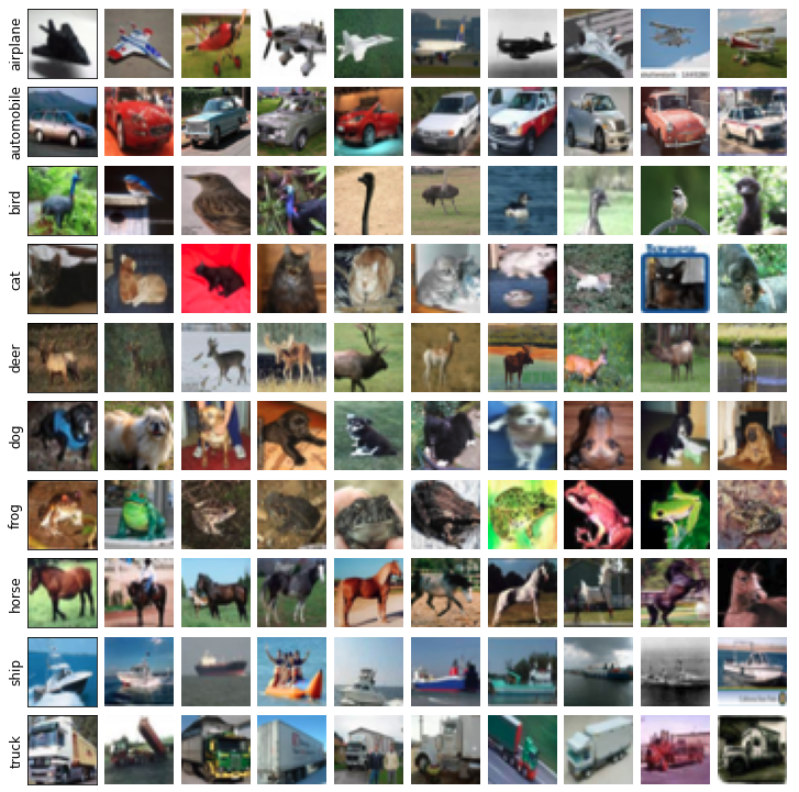
FashionMNIST 데이터셋에서 무작위로 이미지를 9개 가져와서 시각화해보면 아래와 같습니다.
## Iterating and Visualizing the Dataset
import matplotlib.pyplot as plt

labels_map = {
    0: "T-Shirt",
    1: "Trouser",
    2: "Pullover",
    3: "Dress",
    4: "Coat",
    5: "Sandal",
    6: "Shirt",
    7: "Sneaker",
    8: "Bag",
    9: "Ankle Boot",
}

figure = plt.figure(figsize=(8, 8))
cols, rows = 3, 3

for i in range(1, cols * rows + 1):
    sample_idx = torch.randint(len(training_data), size=(1,)).item()
    img, label = training_data[sample_idx]
    figure.add_subplot(rows, cols, i)
    plt.title(labels_map[torch.argmax(label).item()])
    plt.axis("off")
    plt.imshow(img.squeeze(), cmap="gray")
plt.show()

2. DataLoader 를 사용해서 Iterate 하기
모델 학습을 할 때 보통 mini-batch 만큼의 데이터셋을 가져와서 iteration을 돌면서 학습을 진행합니다. 이때 batch_size 만큼 mini-batch 만큼 데이터셋 가져오기, shuffle=True 를 설정해서 무작위로 데이터 가져오기 설정을 할 수 있습니다.
## Preparing your data for training with DataLoaders
from torch.utils.data import DataLoader

train_dataloader = DataLoader(training_data, batch_size=64, shuffle=True)
test_dataloader = DataLoader(test_data, batch_size=64, shuffle=True)


# Display image and label.
train_features, train_labels = next(iter(train_dataloader))
print(f"Feature batch shape: {train_features.size()}")
print(f"Labels batch shape: {train_labels.size()}")
img = train_features[0].squeeze()
label = train_labels[0]
plt.imshow(img, cmap="gray")
plt.show()
print(f"Label: {label}")

# Feature batch shape: torch.Size([64, 1, 28, 28])
# Labels batch shape: torch.Size([64])
# Label: 9
[Reference]
(1) PyTorch Datasets & DataLoaders
: https://pytorch.org/tutorials/beginner/basics/data_tutorial.html
Datasets & DataLoaders — PyTorch Tutorials 2.2.0+cu121 documentation
Note Click here to download the full example code Learn the Basics || Quickstart || Tensors || Datasets & DataLoaders || Transforms || Build Model || Autograd || Optimization || Save & Load Model Datasets & DataLoaders Code for processing data samples can
pytorch.org
(2) PyTorch Transforms
: https://pytorch.org/tutorials/beginner/basics/transforms_tutorial.html
Transforms — PyTorch Tutorials 2.2.0+cu121 documentation
Note Click here to download the full example code Learn the Basics || Quickstart || Tensors || Datasets & DataLoaders || Transforms || Build Model || Autograd || Optimization || Save & Load Model Transforms Data does not always come in its final processed
pytorch.org
이번 포스팅이 많은 도움이 되었기를 바랍니다.
행복한 데이터 과학자 되세요! :-)

'Deep Learning (TF, Keras, PyTorch) > PyTorch basics' 카테고리의 다른 글
| [PyTorch] 모델을 저장하고, 다시 로딩하기 (Saving and Loading the model) (0) | 2023.12.17 |
|---|---|
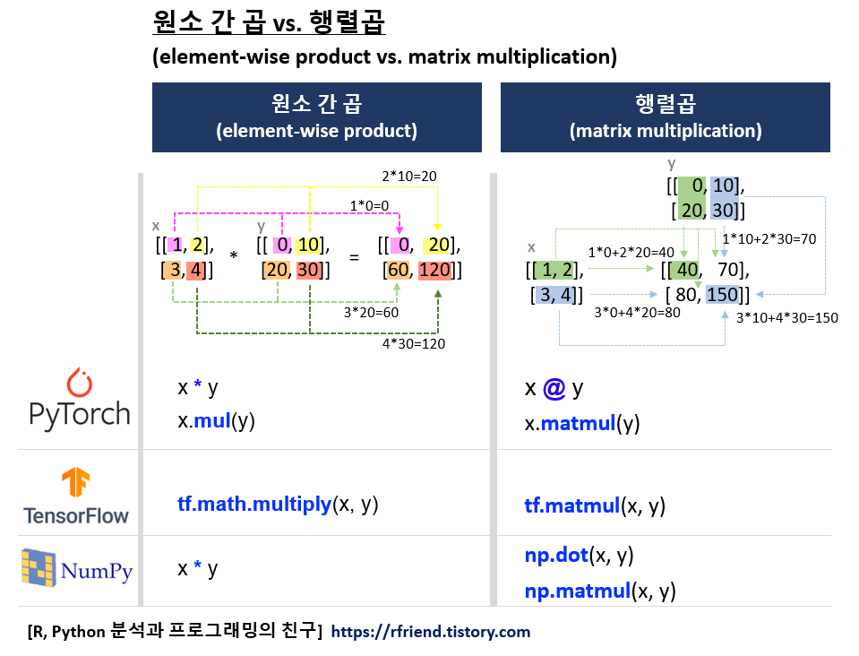
| [PyTorch] 원소 간 곱 vs. 행렬곱 (element-wise product vs. matrix multiplication) (0) | 2023.12.16 |
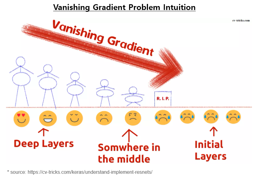
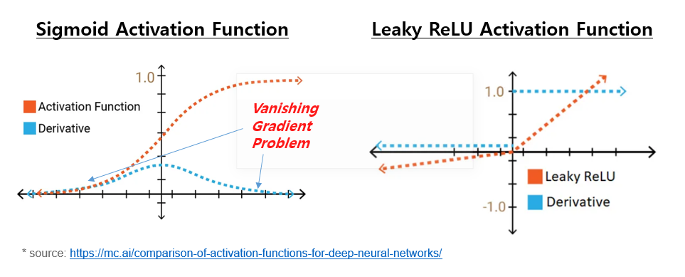
| 기울기 소실 문제(Vanishing Gradient Problem)란 무엇이고, 어떻게 완화할 수 있나? (0) | 2023.12.13 |
| 딥러닝에서 오차역전파법 (Backpropagation, Backward Propagation of Errors) 이란? (0) | 2023.12.12 |
| [PyTorch] torchvision.datasets 모듈에 내장되어 있는 데이터 가져와서 시각화하기 (0) | 2023.02.26 |