[PyTorch] 모델을 저장하고, 다시 로딩하기 (Saving and Loading the model)
Deep Learning (TF, Keras, PyTorch)/PyTorch basics 2023. 12. 17. 10:44이번 포스팅에서는 PyTorch에서 모델을 저장하고 다시 로딩하는 3가지 방법을 소개하겠습니다.
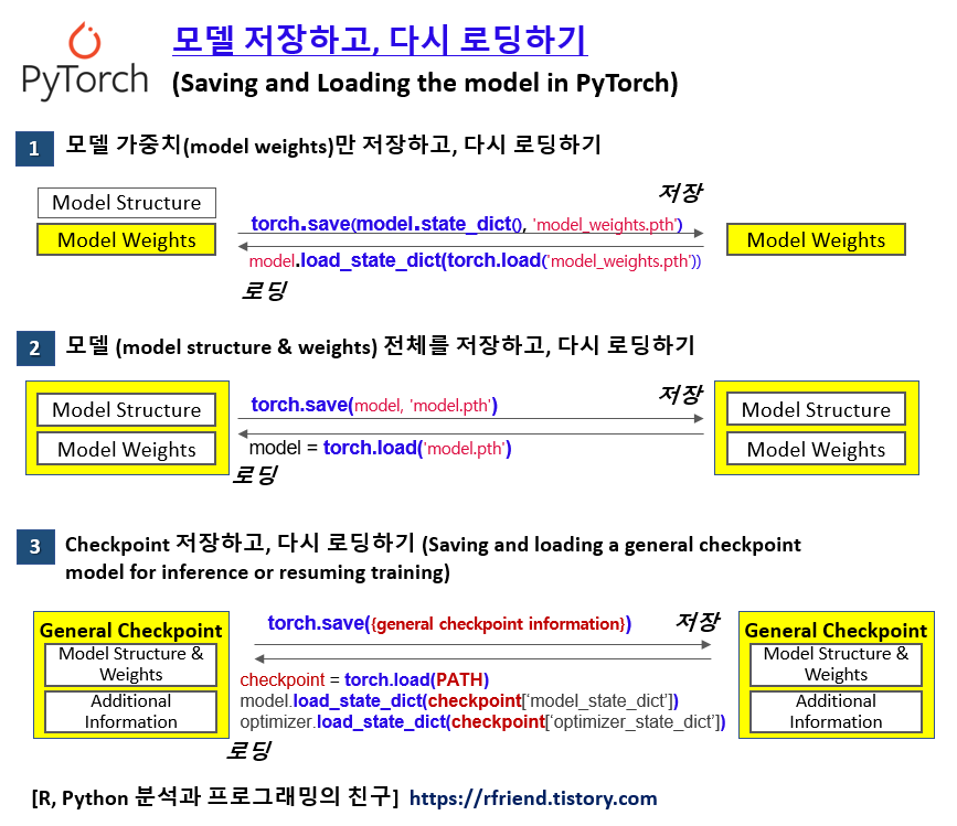
(1) 모델 가중치(model weights) 만 저장하고, 다시 로딩하기
(2) 모델 전체 (model structure & weights) 를 저장하고, 다시 로딩하기
(3) General Checkpoint 를 저장하고, 다시 로딩하기
위 3가지 방법 중에서 하고자 하는 과업의 상황에 맞게 선택해서 사용하면 되겠습니다.
(1) 모델 가중치(model weights) 만 저장하고, 다시 로딩하기
PyTorch 의 internal state dictionary (state_dict)에 있는 학습된 파라미터의 가중치(weights)를 torch.save(model.state_dict(), 'model_weights.pth') 메소드를 사용해서 저장할 수 있습니다.
import torch
import torchvision.models as models


## Saving and Loading model weights
# : PyTorch models store the learned parameters in an internal state dictionary
# : called 'state_dict'
# : These can be persisted via the 'torch.save' method.

model = models.vgg16(weights='IMAGENET1K_V1')
torch.save(model.state_dict(), 'model_weights.pth')
저장된 파라미터별 가중치를 다시 로딩하서 사용하기 위해서는
먼저, 가중치를 저장했을 때와 동일한 모델의 인스턴스를 생성해 놓고,
==> 그 다음에 load_state_dict() 메소드를 사용해서 가중치를 로딩합니다.
(비유하자면, 철근으로 집의 골격을 먼저 세워 놓고, ==> 그 다음에 시멘트를 붇기)
# to load model weights, we need to create an instance of the same model first
# and then load the parameters using 'load_state_dict()' method.

model = models.vgg16() # create untrained model
model.load_state_dict(torch.load('model_weights.pth'))
model.eval() # to set the dropout and batch normalization layers to evaluation mode
(2) 모델 전체 (model structure & weights) 를 저장하고, 다시 로딩하기
다음 방법으로는 모델의 구조(model structure, shape)과 데이터로 부터 학습된 파라미터별 가중치(model weights)를 model.save() 메소드를 사용해서 한꺼번에 저장하는 방법입니다.
## Saving the model with shape and weights
torch.save(model, 'model.pth')
모델의 구조와 가중치가 한꺼번에 저장이 되었기 때문에, 로딩할 때도 torch.load() 메소드로 한꺼번에 모델 구조와 가중치를 가져와서 사용하면 됩니다.
(* (1)번과는 달리, 모델의 구조에 해당하는 인스턴스 생성 절차 없음)
# loading the model with shape and weights
model = torch.load('model.pth')
(3) General Checkpoint 를 저장하고, 다시 로딩하기
여러번의 Epoch를 반복하면서 모델을 훈련하다가, 중간에 그때까지 학습된 모델과 기타 모델 학습 관련된 정보를 직렬화된 딕셔너리(serialized dictionary)로 저장하고, 다시 불러와서 사용할 수도 있습니다.
예를 들어보자면, 먼저 아래처럼 먼저 신경망 클래스를 정의하고 초기화해서 인스턴스를 생성하겠습니다.
import torch
import torch.nn as nn
import torch.optim as optim
import torch.nn.functional as F


# Define and initialize the neural network
class Net(nn.Module):
    def __init__(self):
        super(Net, self).__init__()
        self.conv1 = nn.Conv2d(3, 6, 5)
        self.pool = nn.MaxPool2d(kernel_size=2, stride=2)
        self.conv2 = nn.Conv2d(6, 16, 5)
        self.fc1 = nn.Linear(16*5*5, 120)
        self.fc2 = nn.Linear(120, 84)
        self.fc3 = nn.Linear(84, 10)

    def forward(self, x):
        x = self.pool(F.relu(self.conv1(x)))
        x = self.pool(F.relu(self.conv2(x)))
        x = x.view(-1, 16*5*5)
        x = F.relu(self.fc1(x))
        x = F.relu(self.fc2(x))
        x = self.fc3(x)

        return x

net = Net()
print(net)
# Net(
#   (conv1): Conv2d(3, 6, kernel_size=(5, 5), stride=(1, 1))
#   (pool): MaxPool2d(kernel_size=2, stride=2, padding=0, dilation=1, ceil_mode=False)
#   (conv2): Conv2d(6, 16, kernel_size=(5, 5), stride=(1, 1))
#   (fc1): Linear(in_features=400, out_features=120, bias=True)
#   (fc2): Linear(in_features=120, out_features=84, bias=True)
#   (fc3): Linear(in_features=84, out_features=10, bias=True)
# )
Optimizer 를 초기화하고, 모델 학습과 관련된 추가 정보로 EPOCH, PATH, LOSS 등도 정의를 해준 후에 torch.save() 메소드에 Dictionary 형태로 저장하고자 하는 항목들을 key: value 에 맞춰서 하나씩 정의해주어서 저장을 합니다.
# initialize the optimizer
optimizer = optim.SGD(net.parameters(), lr=0.001, momentum=0.9)

# save the general checkpoint
# : collect all relevant information and build your dictionary.
# additional information
EPOCH = 5
PATH = "model.pt"
LOSS = 0.4

torch.save({
    'epoch': EPOCH,
    'model_state_dict': net.state_dict(),
    'optimizer_state_dict': optimizer.state_dict(),
    'loss': LOSS,
}, PATH)
위에서 처럼 serialized dictionary 형태로 저장된 General Checkpoint 를 다시 로딩해서 사용할 때는,
먼저 저장했을 때와 동일한 model, optimizer 의 인스턴스를 초기화해서 생성해 놓고,
--> torch.load(PATH) 메소드를 사용해서 checkpoint 를 로딩하고
--> load_state_dict() 메소드를 사용해서 로딩한 checkpoint 로부터 저장되어있던 model과 optimizer를 가져와서 사용합니다.
모델 평가나 예측(inference) 용도로 사용할 때는 반드시 model.eval() 를 사용해서 'evaluation model'로 설정해주어야 합니다. 그렇지 않으면 예측을 할 때마다 dropout 과 batch normalization이 바뀌어서 예측값이 바뀌게 됩니다.
만약 모델 훈련을 계속 이어서 하고자 한다면, model.train() 을 사용해서 'training model'로 설정해서 데이터로 부터 계속 Epoch을 반복하면서 학습을 통해 파라미터의 가중치를 업데이트 해주면 됩니다.
## Load the general checkpoint
# : first initialize the model and optimier, then load the dictionary locally.
model = Net()
optimizer =  optim.SGD(model.parameters(), lr=0.001, momentum=0.9) # initialization first

checkpoint = torch.load(PATH)
model.load_state_dict(checkpoint['model_state_dict'])
optimizer.load_state_dict(checkpoint['optimizer_state_dict'])
epoch = checkpoint['epoch']
loss = checkpoint['loss']

model.eval() #  to set dropout and batch normalization layers to evaluation mode before running inference.
[Reference]
(1) PyTorch tutorial - Save and Load the Model
: https://pytorch.org/tutorials/beginner/basics/saveloadrun_tutorial.html
(2) PyTorch tutorial - Saving and Loading a General Checkpoint in PyTorch
: https://pytorch.org/tutorials/beginner/basics/saveloadrun_tutorial.html
이번 포스팅이 많은 도움이 되었기를 바랍니다.
행복한 데이터 과학자 되세요! :-)