레스터 객체의 행과 열의 일부분을 가져오는 것은 Base R의 '[' 연산자('[' operator) 를 사용합니다. raster_object[i, j] 또는 raster_object[Cell_IDs] 구문으로 i행과 j 열을 가져올 수 있습니다. 레스터 객체로 부터 일부분 가져오기는 '(a) 지리정보가 아닌 속성 정보를 가져오기(non-spatial subsetting)'와, '(b) 지리정보 가져오기 (spatial subsetting)' 의 두가지 유형으로 나눌 수 있는데요, 이번 포스팅은 '(a) 레스터 객체로부터 지리정보가 아닌 속성 정보를 가져오기'에 대해서만 다루겠습니다.
elev[1, 1] 은 evel 레스터 객체로 부터 1행과 1열에 위치한 픽셀(pixel, cell) 에 위치한 속성 값을 가져온 것입니다.
elev[1] 은 Cell ID 1번에 위치한 속성 값을 가져온 것입니다. (R 레스터는 좌측 상단에서 부터 1행 1열, Cell ID 1번이 시작하므로 elev[1, 1] 과 elev[1] 은 동일한 위치의 픽셀 속성 값을 가져옴)
## -- (1) Raster subsetting is done with the base R operator '['
## , which accepts a variety of inputs:
## - non-spatial subsetting: row-column indexing, cell IDs
## - spatial subsetting: coordinates, another spatial object

## subsetting the value of the top left pixel in the raster object 'elev'
## (1-1) row-column indexing
elev[1, 1]
# [1] 1

## (1-2) cell IDs
elev[1]
# [1] 1
레스터 객체의 전체 속성 값을 Cell ID의 순서대로 모두 가져오고 싶으면 values(), getValues() 함수 또는 [] 연산자를 사용하면 됩니다.
(2) 다층 레스터 객체(multi-layered laster objects)로 부터 일부 층(layers) 가져오기
(subsetting layers from multi-layered laster objects, a raster brick or stack)
다층 레스터 객체(multi-layered laster objects)로는 RasterBrick 클래스와 RasterStack 클래스가 있습니다. (자세한 설명은 rfriend.tistory.com/617 를 참고하세요.) 이들 다층 레스터 객체로 부터 특정 층을 가져오려면 raster 패키지의 subset() 함수를 사용합니다.
먼저, 예제로 사용할 수 있도록 grain 이라는 레스터 객체를 하나 더 만들고, 이를 (1)에서 만들었던 elev 레스터 객체에 stack() 함수로 쌓아서 다층 레스터 객체를 만들어보겠습니다.
values() 로 r_stack 안의 각 층별 속성값을 조회해보면 아래처럼 "elev" 층과 "grain" 층의 각 Cell 별로 들어있는 속성 값이 들어있음을 알 수 있습니다. (values(r_stack), getValues(r_stack), r_stack[] 모두 동일하게 각 층의 모든 속성값을 반환합니다.)
(3) 레스터 객체의 일부 값을 수정하기 (modifying values in raster objects)
만약 레스터 객체의 일부 값을 새로운 값으로 덮어쓰기, 업데이트, 수정을 하고 싶으면 앞에서 소개한 subsetting 기능을 활용해서 원하는 위치의 행과 열, 픽셀 ID(Pixel ID, Cell ID) 또는 층(layer) 의 subsetting 한 부분에 새로운 속성 값을 할당(<-, =) 하면 됩니다.
아래의 첫번째 예는 elev[1, 1] <- 0 은 elev 레스터 객체의 1행 1열 위치의 셀에 새로운 값 '0'을 할당한 것입니다.
아래의 두번째 예는 evel[1, 1:3] <- 0 은 elev 레스터 객체의 1행의 1~3열 위치 셀에 새로운 값 '0'을 할당하여 속성값을 수정한 것입니다.
이번 포스팅부터는 레스터 객체 데이터셋을 조작하는 방법(manipulating raster objects dataset)을 몇 개의 포스팅으로 나누어서 소개하겠습니다.
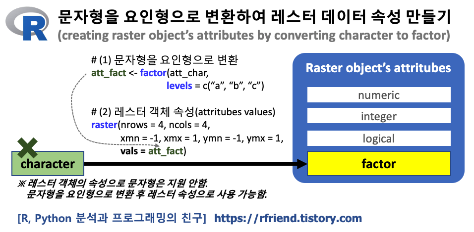
그 중에서도 이번 포스팅에서는 R 문자형을 요인형으로 변환하여 레스터 객체 데이터의 속성으로 만드는 방법(making raster objects attributes by converting character to factor type)을 알아보겠습니다.
R raster objects' attritubes with numeric, integer, logical and factor types. No support for character.
R의 레스터 객체(raster objects)는 데이터 속성으로 숫자형(numeric), 정수형(integer), 논리형(logical), 요인형(factor) 데이터 유형을 지원하며, 문자형(character)은 지원하지 않습니다. 따라서 문자형으로 이루어진 범주형 변수 값(categorical variables' values)을 가지고 레스터 객체의 속성(attritubes)을 만들고 싶으면 (1) 먼저 문자형을 요인형으로 변환 (또는 논리형으로 변환)하고, --> (2) 요인형 값을 속성 값으로 해서 레스터 객체를 만들어야 합니다.
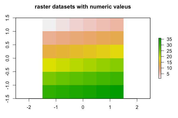
먼저, 레스터 객체 데이터에 대한 이해를 돕기위해, 정수형(integer) 값을 속성 값으로 가지는 레스터 객체를 raster 패키지의 raster() 함수를 사용해서 만들어보겠습니다. 아래의 예에서는 6 x 6 = 36개의 픽셀(pixels, cells)에, x와 y의 좌표값의 최소~최대값 범위의 좌표에, 1~36까지의 정수를 속성 값으로 가지는 레스터 객체 데이터 입니다.
## ========================================================
## R GeoSpatial data analysis
## : Manipulating Raster Objects
## [reference] https://geocompr.robinlovelace.net/attr.html
## ========================================================

## raster data represent continuous surfaces.
## Because of their unique structure,
## subsetting and other operations on raster datasets work in a different way.

library(raster)

## -- creating an example raster dataset
elev <- raster(nrows = 6, # integer > 0. Number of rows
               ncols = 6, # integer > 0. Number of columns
               #res = 0.5, # numeric vector of length 1 or 2 to set the resolution
               xmn = -1.5, # minimum x coordinate (left border)
               xmx = 1.5,  # maximum x coordinate (right border)
               ymn = -1.5, # minimum y coordinate (bottom border)
               ymx = 1.5,  # maximum y coordinate (top border)
               vals = 1:36) # values for the new RasterLayer

elev
# class      : RasterLayer
# dimensions : 6, 6, 36  (nrow, ncol, ncell)
# resolution : 0.5, 0.5  (x, y)
# extent     : -1.5, 1.5, -1.5, 1.5  (xmin, xmax, ymin, ymax)
# crs        : +proj=longlat +datum=WGS84 +no_defs
# source     : memory
# names      : layer
# values     : 1, 36  (min, max)


plot(elev, main = 'raster datasets with numeric valeus')
이제 본론으로 넘어가서, 문자형으로 이루어진 범주형 변수를 요인형으로 변환한 후에, 이를 다시 레스터 객체의 속성으로 하여 레스터 객체를 만드는 방법을 소개하겠습니다.
(1)
문자형(character)을 요인형(factor)으로 변환할 때는 R base 패키지의 factor() 를 사용합니다. 이때 요인의 수준(levels)은 범주형 변수 내 유일한(unique) 문자열을 오름차순으로 정렬(sorting in an increasing order)하여 부여가 되는데요, 만약 요인의 수준(levels)을 특정 순서에 맞게 분석가가 수작업으로 설정을 하고 싶다면 levels 매개변수를 사용해서 직접 요인 수준을 입력을 해주면 됩니다.
아래 예에서는 모래의 굵기의 수준에 따라서 "점토(clay)", "미세모래(silt)", "모래(sand)"의 순서로 levels 매개변수를 이용해 요인의 수준을 설정해서, factor() 함수로 문자형으로 구성된 범주형 변수('grain_order')를 요인형 변수('grain_fact')으로 변환해준 것입니다.
<--> 만약 factor() 함수로 요인형으로 변환할 때 levels 매개변수로 요인 수준의 순서를 지정해주지 않는다면, default 인 유일한 문자형 값들의 오름차순 정렬에 따라서 ["clay", "sand", "silt"] 의 순서로 설정이 되었을 것입니다.
## -- raster objects can contain values of class numeric, integer, logical or factor,
## but not character.
## Raster objects can also contain categorical values of
## class logical or factor variables in R.


grain_order <- c("clay", "silt", "sand")

## random sampling with replacement
set.seed(1004)
grain_char <- sample(grain_order, 36, replace = TRUE)
grain_char
# [1] "sand" "silt" "clay" "clay" "clay" "sand" "silt" "silt" "silt" "clay" "sand" "silt" "sand" "sand"
# [15] "sand" "clay" "sand" "clay" "sand" "clay" "sand" "sand" "silt" "clay" "sand" "silt" "sand" "clay"
# [29] "clay" "clay" "sand" "sand" "clay" "sand" "sand" "clay"


## converting character into factor
grain_fact <- factor(grain_char,
                     # ordered factor: clay < silt < sand in terms of grain size.
                     levels = grain_order)

grain_fact
# [1] sand silt clay clay clay sand silt silt silt clay sand silt sand sand sand clay sand clay sand clay
# [21] sand sand silt clay sand silt sand clay clay clay sand sand clay sand sand clay
# Levels: clay silt sand
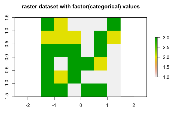
(2) 요인형 값을 속성으로 한 레스터 객체 데이터 만들기 (creating raster objects with factor values)
위의 (1)번에서 문자열 값을 요인형으로 변환한 값을 가지고 raster 패키지의 raster() 함수를 사용해서 레스터 객체를 만들어보겠습니다. 행의 수(nrows) 6개, 열의 수(ncols) 6개의 총 36개 픽셀(pixcels, cells)을 가지는 레스터 객체에 raster(nrows = 6, ncols = 6, res = 0.5, vals = grain_fact)('grain_fact' 는 요인형 값을 가지는 벡터임) 을 입력하였습니다.
레스터 객체 데이터에 대해서 plot() 함수로 간단하게 시각화를 할 수 있습니다. 이때 요인형의 수준 값(levels)인 clay = 1, silt = 2, sand = 3 의 정수값을 가지고 시각화를 하게 됩니다.
이번에는 levels() 와 cbind() 함수를 사용해서 기존의 요인의 수준에다가 wetness = c("wet", "moist", "dry") 라는 새로운 요인 수준을 추가(adding new factor levels to the attritube table) 하여 보겠습니다.
## -- Use the function levels() for retrieving and
##    adding new factor levels to the attribute table:
levels(grain_raster)
# [[1]]
# ID VALUE
# 1  1  clay
# 2  2  silt
# 3  3  sand

## adding new factor levels
levels(grain_raster)[[1]] = cbind(levels(grain_raster)[[1]],
                                  wetness = c("wet", "moist", "dry"))


## retrieving factor levels
levels(grain_raster)
# [[1]]
# ID VALUE wetness
# 1  1  clay     wet
# 2  2  silt   moist
# 3  3  sand     dry
레스터 객체 데이터의 "attritubes"라는 이름의 속성 테이블(attritube table)에 요인형 수준 값이 저장되어 있으며, 여기에 새로운 요인형 수준 값이 추가되는 것입니다. ratify() 함수를 사용하면 이 속성 테이블(attritube table)에 저장되어 있는 값을 조회할 수 있습니다.
## -- The raster object stores the corresponding look-up table
## or “Raster Attribute Table” (RAT) as a data frame in a new slot named attributes,
## which can be viewed with ratify(grain)

ratify(grain_raster)
# class      : RasterLayer
# dimensions : 6, 6, 36  (nrow, ncol, ncell)
# resolution : 0.5, 0.5  (x, y)
# extent     : -1.5, 1.5, -1.5, 1.5  (xmin, xmax, ymin, ymax)
# crs        : +proj=longlat +datum=WGS84 +no_defs
# source     : memory
# names      : layer
# values     : 1, 3  (min, max)
# attributes :
#   ID
# 1
# 2
# 3
레스터 객체의 각 픽셀(pixcel, cell)은 단 하나의 값만을 가질 수 있습니다. 이 예제에서는 각 픽셀이 하나의 요인 수준 값을 가지고 있는데요, 아래 예는 레스터 객체의 1번, 10번, 26번 픽셀의 요인 수준 값이 3, 1, 2 이고, 이들 요인 수준 값에 대응하는 속성 정보를 factorValues() 함수를 사용하여 속성 테이블(attritube table) 로 부터 매핑하여 보여주는 것입니다.
## -- looking up the attributes in the corresponding attribute table
grain_raster[c(1, 10, 26)]
# [1] 3 1 2

factorValues(grain_raster, grain_raster[c(1, 10, 26)])
# VALUE wetness
# 1  sand     dry
# 2  clay     wet
# 3  silt   moist
지난번 포스팅에서는 지리 벡터 데이터의 두 테이블의 Join Key 를 정규표현식을 사용한 패턴 매칭을 통해 일치를 시킨 후에 두 데이터 테이블을 Join 하는 방법(rfriend.tistory.com/626)을 소개하였습니다.
이번 포스팅에서는 sf 클래스의 지리 벡터 데이터에서 Base R, dplyr, tidyr 의 R 패키지를 이용하여 기존 속성을 가지고 새로운 속성을 만드는 방법과, 지리 정보(spatial information)을 제거하는 방법을 소개하겠습니다.
(1) Base R 로 지리 벡터 데이터에 새로운 속성 만들기
(2) dplyr 로 지리 벡터 데이터에 새로운 속성 만들기 : mutate(), transmute()
(3) tidyr 로 지리 벡터 데이터의 기존 속성을 합치거나 분리하기 : unite(), separate()
(4) dplyr 로 지리 벡터 데이터의 속성 이름 바꾸기 : rename(), setNames()
(5) 지리 벡터 데이터에서 지리 정보 제거하기 : st_drop_geometry()
(1) Base R 로 지리 벡터 데이터에 새로운 속성 만들기
먼저 예제로 사용할 sf 클래스 객체 데이터셋으로는, spData 패키지에 내장된 "world" 데이터셋을 사용하겠습니다. "world" 데이터셋에는 177개 국가의 지리기하 geometry 정보를 포함하고 있으며, sf 클래스를 사용하여 지리공간 데이터 처리 및 분석을 할 수 있습니다. 원래의 데이터를 덮어쓰지 않기 위해 "world_new" 라는 복사 데이터셋을 추가로 하나 더 만들었습니다. 그리고 데이터 전처리를 위해 dplyr, tidyr 패키지를 불러오겠습니다.
## =============================================================
## GeoSpatial data analysis using R
## : Creating vector attributes and removing spatial information
## : reference: https://geocompr.robinlovelace.net/attr.html
## =============================================================

library(sf)
library(spData)
library(dplyr) # mutate(), transmute()
library(tidyr) # unite(), separate()

str(world)
# tibble [177 x 11] (S3: sf/tbl_df/tbl/data.frame)
# $ iso_a2   : chr [1:177] "FJ" "TZ" "EH" "CA" ...
# $ name_long: chr [1:177] "Fiji" "Tanzania" "Western Sahara" "Canada" ...
# $ continent: chr [1:177] "Oceania" "Africa" "Africa" "North America" ...
# $ region_un: chr [1:177] "Oceania" "Africa" "Africa" "Americas" ...
# $ subregion: chr [1:177] "Melanesia" "Eastern Africa" "Northern Africa" "Northern America" ...
# $ type     : chr [1:177] "Sovereign country" "Sovereign country" "Indeterminate" "Sovereign country" ...
# $ area_km2 : num [1:177] 19290 932746 96271 10036043 9510744 ...
# $ pop      : num [1:177] 8.86e+05 5.22e+07 NA 3.55e+07 3.19e+08 ...
# $ lifeExp  : num [1:177] 70 64.2 NA 82 78.8 ...
# $ gdpPercap: num [1:177] 8222 2402 NA 43079 51922 ...
# $ geom     :sfc_MULTIPOLYGON of length 177; first list element: List of 3
# ..$ :List of 1
# .. ..$ : num [1:8, 1:2] 180 180 179 179 179 ...
# ..$ :List of 1
# .. ..$ : num [1:9, 1:2] 178 178 179 179 178 ...
# ..$ :List of 1
# .. ..$ : num [1:5, 1:2] -180 -180 -180 -180 -180 ...
# ..- attr(*, "class")= chr [1:3] "XY" "MULTIPOLYGON" "sfg"
# - attr(*, "sf_column")= chr "geom"
# - attr(*, "agr")= Factor w/ 3 levels "constant","aggregate",..: NA NA NA NA NA NA NA NA NA NA
# ..- attr(*, "names")= chr [1:10] "iso_a2" "name_long" "continent" "region_un" ...


## do not overwrite the original data
world_new = world
sf 클래스 객체의 속성(Attributes)에 대해서 Base R 의 기본 구문인 '$' 와 '=', '<-' 을 사용해서 새로운 속성을 만들 수 있습니다.
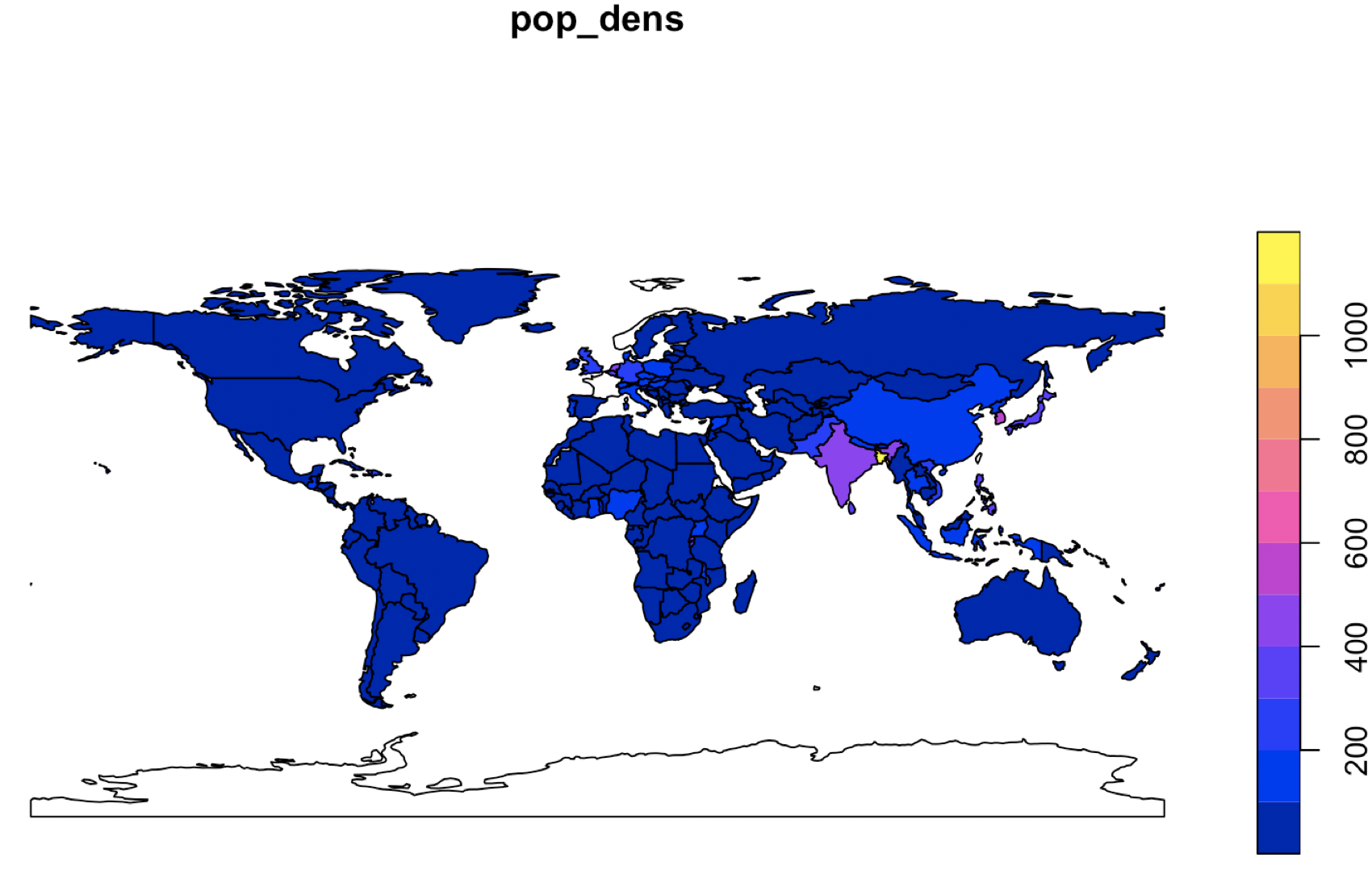
가령, 국가별 인구("pop")를 면적("area_km2")로 나누어서 '(km2 면적 당) 인구밀도("pop_dens")' 라는 새로운 속성을 만들어 보겠습니다. 새로운 속성 칼럼인 "pop_dens"가 생성이 된 후에도 "world_new" 데이터셋은 sf 클래스 객체의 특성을 계속 유지하고 있습니다. 따라서 plot(world_new["pop_dens"] 로 시각화를 하면, 아래와 같이 다면 (multi-polygons) 기하로 표현되는 세계 국가별 지도 위에, 기존 칼럼을 사용해 계산해서 새로 만든 속성 칼럼인 '인구밀도("pop_dens")' 를 시각화할 수 있습니다.
## creating new column using Base R
world_new$pop_dens = world_new$pop / world_new$area_km2


## attribute data operations preserve the geometry of the simple features
## plot() will visualize map using geometry
plot(world_new['pop_dens'])
(2) dplyr 로 지리 벡터 데이터에 새로운 속성 만들기 : mutate(), transmute()
위 (1)번의 Base R 대비 dplyr 를 사용하면, 한꺼번에 여러개의 신규 속성 칼럼을 생성할 수 있고, 체인('%>%')을 이용해서 파이프 연산자로 이전 작업 결과를 다음 작업으로 넘겨주는 방식으로 작업 흐름을 코딩할 수 있어 가독성이 뛰어난 코드를 짤 수 있는 장점이 있습니다.
mutate() 함수는 기존 데이터셋에 새로 만든 데이터셋을 추가해주는 반면에, transmute() 함수는 기존의 칼럼은 모두 제거를 하고 새로 만든 칼럼과 지리기하 geometry 칼럼만을 반환합니다. (이때 sf 클래스 객체의 경우 '지리기하 geometry 칼럼'이 껌딱지처럼 달라붙어서 계속 따라 다닌다는 점이 중요합니다!)
## creating new columns using dplyr
world %>%
  mutate(pop_dens = pop / area_km2)

# Simple feature collection with 177 features and 11 fields
# geometry type:  MULTIPOLYGON
# dimension:      XY
# bbox:           xmin: -180 ymin: -90 xmax: 180 ymax: 83.64513
# geographic CRS: WGS 84
# # A tibble: 177 x 12
# iso_a2 name_long  continent  region_un subregion type  area_km2     pop lifeExp gdpPercap                        geom pop_dens
# * <chr>  <chr>      <chr>      <chr>     <chr>     <chr>    <dbl>   <dbl>   <dbl>     <dbl> <MULTIPOLYGON [arc_degree]>    <dbl>
# 1 FJ     Fiji       Oceania    Oceania   Melanesia Sove~   1.93e4  8.86e5    70.0     8222. (((180 -16.06713, 180 -16.~    45.9
# 2 TZ     Tanzania   Africa     Africa    Eastern ~ Sove~   9.33e5  5.22e7    64.2     2402. (((33.90371 -0.95, 34.0726~    56.0
# 3 EH     Western S~ Africa     Africa    Northern~ Inde~   9.63e4 NA         NA         NA  (((-8.66559 27.65643, -8.6~    NA
# 4 CA     Canada     North Ame~ Americas  Northern~ Sove~   1.00e7  3.55e7    82.0    43079. (((-122.84 49, -122.9742 4~     3.54
# 5 US     United St~ North Ame~ Americas  Northern~ Coun~   9.51e6  3.19e8    78.8    51922. (((-122.84 49, -120 49, -1~    33.5
# 6 KZ     Kazakhstan Asia       Asia      Central ~ Sove~   2.73e6  1.73e7    71.6    23587. (((87.35997 49.21498, 86.5~     6.33
# 7 UZ     Uzbekistan Asia       Asia      Central ~ Sove~   4.61e5  3.08e7    71.0     5371. (((55.96819 41.30864, 55.9~    66.7
# 8 PG     Papua New~ Oceania    Oceania   Melanesia Sove~   4.65e5  7.76e6    65.2     3709. (((141.0002 -2.600151, 142~    16.7
# 9 ID     Indonesia  Asia       Asia      South-Ea~ Sove~   1.82e6  2.55e8    68.9    10003. (((141.0002 -2.600151, 141~   140.
# 10 AR     Argentina  South Ame~ Americas  South Am~ Sove~   2.78e6  4.30e7    76.3    18798. (((-68.63401 -52.63637, -6~    15.4
# # ... with 167 more rows
transmute() 함수를 사용해서 '(km2 면적당) 인구밀도 ("pop_dens")' 의 신규 속성을 만들면, 기존의 속성 칼럼들은 모두 제거 되고 새로운 '인구밀도' 속성 칼럼과 '지리기하 geom' 칼럼만 남게 됩니다.
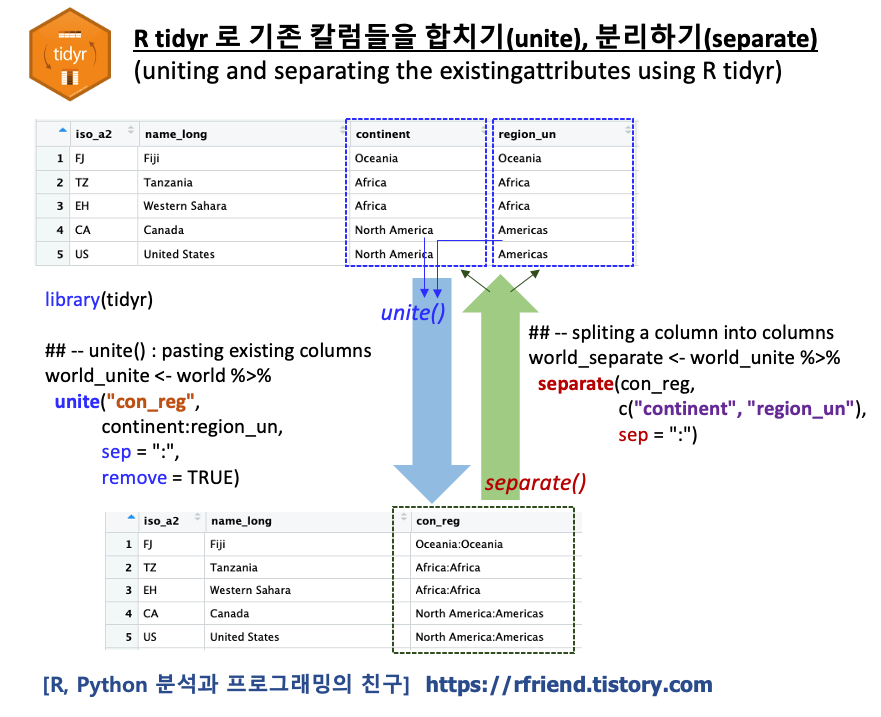
(3) tidyr 로 지리 벡터 데이터의 기존 속성을 합치거나 분리하기 : unite(), separate()
tidyr 패키지에 있는 unite(data, col, lll, sep = "_", remove = TRUE) 함수를 사용하면 기존의 속성 칼럼을 합쳐서 새로운 속성 칼럼을 만들 수 있습니다. 이때 remove = TRUE 매개변수를 설정해주면 기존의 합치려는 두 개의 칼럼은 제거되고, 새로 만들어진 칼럼만 남게 됩니다.
## -- unite(): pasting together existing columns.
library(tidyr)

world_unite = world %>%
  unite("con_reg", continent:region_un,
        sep = ":",
        remove = TRUE)

world_unite
# Simple feature collection with 177 features and 9 fields
# geometry type:  MULTIPOLYGON
# dimension:      XY
# bbox:           xmin: -180 ymin: -90 xmax: 180 ymax: 83.64513
# geographic CRS: WGS 84
# # A tibble: 177 x 10
# iso_a2 name_long   con_reg     subregion    type    area_km2     pop lifeExp gdpPercap                                    geom
# <chr>  <chr>       <chr>       <chr>        <chr>      <dbl>   <dbl>   <dbl>     <dbl>             <MULTIPOLYGON [arc_degree]>
# 1 FJ     Fiji        Oceania:Oc~ Melanesia    Sovere~   1.93e4  8.86e5    70.0     8222. (((180 -16.06713, 180 -16.55522, 179.3~
# 2 TZ     Tanzania    Africa:Afr~ Eastern Afr~ Sovere~   9.33e5  5.22e7    64.2     2402. (((33.90371 -0.95, 34.07262 -1.05982, ~
# 3 EH     Western Sa~ Africa:Afr~ Northern Af~ Indete~   9.63e4 NA         NA         NA  (((-8.66559 27.65643, -8.665124 27.589~
# 4 CA     Canada      North Amer~ Northern Am~ Sovere~   1.00e7  3.55e7    82.0    43079. (((-122.84 49, -122.9742 49.00254, -12~
# 5 US     United Sta~ North Amer~ Northern Am~ Country   9.51e6  3.19e8    78.8    51922. (((-122.84 49, -120 49, -117.0312 49, ~
# 6 KZ     Kazakhstan  Asia:Asia   Central Asia Sovere~   2.73e6  1.73e7    71.6    23587. (((87.35997 49.21498, 86.59878 48.5491~
# 7 UZ     Uzbekistan  Asia:Asia   Central Asia Sovere~   4.61e5  3.08e7    71.0     5371. (((55.96819 41.30864, 55.92892 44.9958~
# 8 PG     Papua New ~ Oceania:Oc~ Melanesia    Sovere~   4.65e5  7.76e6    65.2     3709. (((141.0002 -2.600151, 142.7352 -3.289~
# 9 ID     Indonesia   Asia:Asia   South-Easte~ Sovere~   1.82e6  2.55e8    68.9    10003. (((141.0002 -2.600151, 141.0171 -5.859~
# 10 AR     Argentina   South Amer~ South Ameri~ Sovere~   2.78e6  4.30e7    76.3    18798. (((-68.63401 -52.63637, -68.25 -53.1, ~
# # ... with 167 more rows
tidyr 패키지의 separate(data, col, sep = "[^:alnum:]]+", remove = TRUE, ...) 함수는 기존에 존재하는 칼럼을 구분자(sep)를 기준으로 두 개의 칼럼으로 분리(separation, splitting)를 해줍니다. 이때 remove = TRUE 매개변수를 설정해주면 기존의 분리하려는 원래 속성 칼럼은 제거가 됩니다.
역시, unite() 또는 separate() 함수 적용 후의 결과 데이터셋은 sf 클래스 객체로서, 제일 뒤에 지리기하 geometry 칼럼이 계속 붙어 있습니다.
## -- separate(): splitting one column into multiple columns
## : using either a regular expression or character positions.
world_separate <- world_unite %>%
  separate(con_reg,
           c("continent", "region_un"),
           sep = ":")


world_separate
# Simple feature collection with 177 features and 10 fields
# geometry type:  MULTIPOLYGON
# dimension:      XY
# bbox:           xmin: -180 ymin: -90 xmax: 180 ymax: 83.64513
# geographic CRS: WGS 84
# # A tibble: 177 x 11
#    iso_a2 name_long  continent  region_un subregion   type   area_km2     pop lifeExp gdpPercap                              geom
#    <chr>  <chr>      <chr>      <chr>     <chr>       <chr>     <dbl>   <dbl>   <dbl>     <dbl>       <MULTIPOLYGON [arc_degree]>
#  1 FJ     Fiji       Oceania    Oceania   Melanesia   Sover~   1.93e4  8.86e5    70.0     8222. (((180 -16.06713, 180 -16.55522,~
#  2 TZ     Tanzania   Africa     Africa    Eastern Af~ Sover~   9.33e5  5.22e7    64.2     2402. (((33.90371 -0.95, 34.07262 -1.0~
#  3 EH     Western S~ Africa     Africa    Northern A~ Indet~   9.63e4 NA         NA         NA  (((-8.66559 27.65643, -8.665124 ~
#  4 CA     Canada     North Ame~ Americas  Northern A~ Sover~   1.00e7  3.55e7    82.0    43079. (((-122.84 49, -122.9742 49.0025~
#  5 US     United St~ North Ame~ Americas  Northern A~ Count~   9.51e6  3.19e8    78.8    51922. (((-122.84 49, -120 49, -117.031~
#  6 KZ     Kazakhstan Asia       Asia      Central As~ Sover~   2.73e6  1.73e7    71.6    23587. (((87.35997 49.21498, 86.59878 4~
#  7 UZ     Uzbekistan Asia       Asia      Central As~ Sover~   4.61e5  3.08e7    71.0     5371. (((55.96819 41.30864, 55.92892 4~
#  8 PG     Papua New~ Oceania    Oceania   Melanesia   Sover~   4.65e5  7.76e6    65.2     3709. (((141.0002 -2.600151, 142.7352 ~
#  9 ID     Indonesia  Asia       Asia      South-East~ Sover~   1.82e6  2.55e8    68.9    10003. (((141.0002 -2.600151, 141.0171 ~
# 10 AR     Argentina  South Ame~ Americas  South Amer~ Sover~   2.78e6  4.30e7    76.3    18798. (((-68.63401 -52.63637, -68.25 -~
# # ... with 167 more rows
(4) dplyr 로 지리 벡터 데이터의 속성 이름 바꾸기 : rename(), setNames()
dplyr 패키지로 sf 객체이자 data frame 인 데이터셋의 특정 속성 변수 이름을 바꾸려면 rename(data, new_name = old_name) 함수를 사용합니다.
만약 여러개의 속성 칼럼 이름을 한꺼번에 변경, 혹은 부여하고 싶다면 stats 패키지의 setNames(object = nm, nm) 함수를 dplyr의 체인 파이프 라인에 같이 사용하면 편리합니다.
##-- setNames() changes all column names at once
new_names <- c("i", "n", "c", "r", "s", "t", "a", "p", "l", "gP", "geom")

world_setnm <- world %>%
  setNames(new_names)

names(world_setnm)
# [1] "i"    "n"    "c"    "r"    "s"    "t"    "a"    "p"    "l"    "gP"   "geom"
(5) 지리 벡터 데이터에서 지리 정보 제거하기 : st_drop_geometry()
위의 (1)~(4)번까지의 새로운 속성 칼럼 생성/ 이름 변경 등의 작업을 하고 난 결과 데이터셋에는 항상 '지리기하 geometry' 칼럼이 착 달라붙어서 따라 다녔습니다. 이게 지리공간 데이터 분석을 할 때 '속성(attributes)' 정보와 '지리기하 geometry' 정보를 같이 연계하여 분석해야 하는 경우에는 매우 유용합니다. 하지만, 경우에 따라서는 '속성'정보만 필요하고 '지리기하 geometry' 정보는 필요하지 않을 수도 있을 텐데요, 이럴때 많은 저장 용량과 처리 부하를 차지하는 '지리기하 geometry' 칼럼은 제거하고 싶을 것입니다. 이때 sf 패키지의 st_drop_geometry() 함수를 사용해서 sf 클래스 객체에 들어있는 '지리기하 geometry' 정보를 제거할 수 있습니다.
## -- st_drop_geometry(): remove the geometry

## "sf" class
class(world)
# [1] "sf"         "tbl_df"     "tbl"        "data.frame"

## "data.frame"
world_data <- world %>% st_drop_geometry()
class(world_data)
# [1] "tbl_df"     "tbl"        "data.frame"
지난번 포스팅에서는 두 개의 sf 클래스 객체의 지리 벡터 데이터 테이블을 R dplyr 패키지의 함수를 사용하여 Mutating Joins, Filtering Joins, Nesting Joins 하는 방법을 소개하였습니다(rfriend.tistory.com/625).
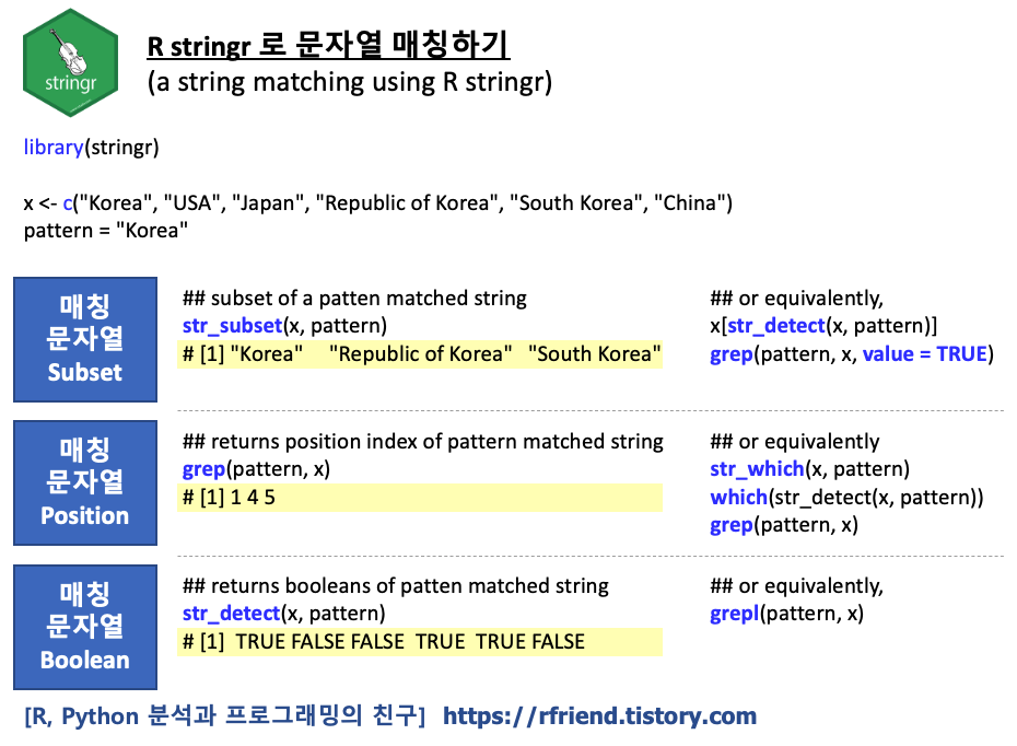
이번 포스팅에서는 여기서 특수한 경우로 조금 더 깊이 들어가서, 두 테이블을 Join 하는 기준이 되는 Key 칼럼이 문자열로 되어 있고, 데이터 표준화가 미흡한 문제로 인해 정확하게 매칭이 안되어서 Join 이 안되는 경우에, R의 stringr 패키지를 사용해 정규 표현식의 문자열 매칭(a string matching using regular expression)으로 Key 값을 변환하여 두 테이블을 Join 하는 방법을 소개하겠습니다.
먼저, 전세계 국가별 지리기하와 속성 정보를 모아놓은 sf 클래스 객체의 지리 벡터 데이터셋인 "world" 와, 2016년과 2017년 국가별 커피 생산량을 집계한 data frame 인 "coffee_data" 의 두 개 데이터셋을 spData 로 부터 가져오겠습니다.
그리고 두 개 테이블 Join 을 위해 dplyr 패키지를 불러오고, 정규 표현식을 이용한 문자열 매칭을 위해 stringr 패키지를 불러오겠습니다.
"world" 데이터셋은 177개의 행(국가)과 11개의 열(속성(attritubes)과 지리기하 칼럼(gemgraphy column)) 으로 이루어져 있습니다. "coffee_data"는 47개의 행과 3개의 열로 구성되어 있습니다.
## =========================================================
## inner join using a string matching
## - reference: https://geocompr.robinlovelace.net/attr.html
## =========================================================

library(sf)
library(spData)
library(dplyr)
library(stringr) # for a string matching

## -- two geography vector dataset tables : world, coffee_data
## -- (a) world: World country pologons in spData
names(world)
# [1] "iso_a2"  "name_long" "continent" "region_un" "subregion" "type"  "area_km2"  "pop"  "lifeExp"   "gdpPercap"
# [11] "geom"

dim(world)
# [1] 177  11


## -- (b) coffee_data: World coffee productiond data in spData
## : estimated values for coffee production in units of 60-kg bags in each year
names(coffee_data)
# [1] "name_long"      "coffee_production_2016" "coffee_production_2017"

dim(coffee_data)
# [1] 47  3
(1) 두 테이블 inner join 하기: inner_join(x, y, by)
"world"와 "coffee_data"의 두개 데이터 테이블을 inner join 해보면 45개의 행(즉, 국가)과 13개의 열(= "world"로 부터 11개의 칼럼 + "coffee_data"로 부터 2개의 칼럼) 으로 이루어진 Join 결과를 반환합니다.
위에서 "coffee_data" 데이터셋이 47개의 행으로 이루어졌다고 했는데요, inner join 한 결과는 행이 45개로서 2개가 서로 차이가 나는군요.
## -- inner join
world_coffee_inner = inner_join(x = world,
                                y = coffee_data,
                                by = "name_long")

## or shortly
world_coffee_inner = inner_join(world, coffee_data)
# Joining, by = "name_long"


dim(world_coffee_inner)
# [1] 45 13


nrow(world_coffee_inner)
# [1] 45
(2) 두 문자열의 원소 차이 알아보고 문자열 매칭으로 찾아보기: setdiff(), str_subset()
Join 전과 후에 어느 국가에서 차이가 나는지 확인해 보기 위해 setdiff() 함수를 사용해서 Join의 Key로 사용이 되었던 'name_long' (긴 국가 이름)에 대해 "coffee_data" 와 "world" 데이터의 원소 간 차이를 구해보았습니다. 그랬더니 ["Congo, Dem. Rep. of", "Others"] 의 2개 'name_long' 에서 차이가 있네요.
다음으로, "world" 의 'name_long' 칼럼의 원소 중에서 "Dem"으로 시작하고 "Congo"를 포함하고 있는 문자열을 stringr 패키지의 str_subset(string, pattern) 함수를 사용해 정규 표현식의 문자열 매칭으로 찾아보겠습니다. "world" 데이터셋의 'name_long' 칼럼에는 "Democratic Republic of the Congo" 라는 이름으로 데이터가 들어가 있네요. ("coffee_data" 데이터셋에는 "Confo, Dem. Rep. of" 라고 들어가 있다보니, 서로 같은 국가임에도 left_join() 을 했을 때 서로 정확하게 매칭이 안되어 Join 이 안되었습니다.)
참고로, str_subset() 은 x[str_detect(x, pattern)] 의 wrapper 입니다. 그리고 grep(pattern, x, value = TRUE) 와 동일한 역할을 수행합니다.
## setdiff(): calculates the set difference of subsets of two data frames
setdiff(coffee_data$name_long, world$name_long)
# [1] "Congo, Dem. Rep. of" "Others"


## string matching (regex) function from the stringr package
str_subset(world$name_long, "Dem*.+Congo")
# [1] "Democratic Republic of the Congo"
(3) 문자열 매칭으로 Key 값 업데이트 하고, 다시 두 테이블 inner join 하기
이제 Join Key로 사용하는 'name_long' 칼럼에서 "Congo" 국가에 대한 표기가 "world" 와 "coffee_data" 의 두 개 데이터셋이 서로 조금 다르다는 이유로 Join 이 안된다는 문제를 해결해 보겠습니다.
grepl(pattern, x) 함수로 "coffee_data" 데이터셋의 'name_long' 칼럼에서 "Congo" 가 들어있는 행을 찾아서, 그 행의 값의 str_subset() 의 정규표현식 문자열 매칭으로 찾은 (str_subset(world$name_long, "Dem*.+Congo") 이름인 "Demogratic Republic of the Congo" 라는 이름으로 대체를 해보겠습니다. 이렇게 하면 "world"와 "coffee_data"에 있는 "Congo" 국가의 긴 이름이 동일하게 "Demogratic Republic of Congo"로 되어 Join 이 제대로 될 것입니다.
## updating 'name_long' values using a string matching
coffee_data$name_long[grepl("Congo", coffee_data$name_long)] =
  str_subset(world$name_long, "Dem*.+Congo")

## inner join again using an updated key
world_coffee_match = inner_join(world, coffee_data)
#> Joining, by = "name_long"

nrow(world_coffee_match)
#> [1] 46
참고로, R에서 문자열 패턴 매칭을 할 때 grepl(pattern, x) 은 패턴 매칭되는 여부에 대해 TRUE, FALSE 로 블러언 값을 반환하는 반면에, grep(pattern, x) 은 패턴 매칭이 되는(TRUE) 위치 인덱스(Position Index)를 반환합니다.
dplyr 패키지로 두 테이블을 Join 할 때 왼쪽(x, LHS, Left Hand Side)에 써주는 테이블의 데이터 구조로 Join 한 결과를 반환합니다. 즉, Join 할 테이블을 써주는 순서가 중요합니다.
가령, 아래의 예에서는 "world" 가 'sf' 클래스의 지리 벡터 객체이고, 'coffee_data'는 tydiverse의 tibble, data.frame 객체입니다. left_join(world, coffee_data) 로 'world' 의 'sf' 지리 벡터 객체를 Join 할 때 왼쪽(LHS, x)에 먼저 써주면 Join 한 결과도 'sf' 클래스의 지리 벡터 객체가 됩니다.(R이 지리공간 벡터 데이터임을 알고 'sf' 클래스를 적용한 지리공간 데이터 처리 및 분석이 가능함).
반면에, left_join(coffee_data, world) 로 'coffee_data'의 'data.frame'을 Join 할 때 왼쪽(LHS, x)에 먼저 써주면 Join 한 결과도 'data.frame' 객체가 반환됩니다. (지리공간 'sf' 클래스가 더이상 아님)
## starting with a non-spatial dataset and
## adding variables from a simple features object.
## the result is not another simple feature object,
## but a data frame in the form of a tidyverse tibble:
## the output of a join tends to match its first argument.

## -- (a) 'sf' object first, then returns 'sf' object.
world_coffee = left_join(world, coffee_data)
#> Joining, by = "name_long"

class(world_coffee)
# [1] "sf"         "tbl_df"     "tbl"        "data.frame"


## -- (b) 'data.frame' object first, then returns 'data.frame' object.
coffee_world = left_join(coffee_data, world)
#> Joining, by = "name_long"

class(coffee_world)
#> [1] "tbl_df"     "tbl"        "data.frame"
(5) data.frame을 'sf' 클래스 객체로 변환하기
'sf' 패키지의 st_as_df() 함수를 사용하면 data.frame 을 'sf' 클래스 객체로 변환할 수 있습니다.
## -- converting data.frame to 'sf' class object

st_as_sf(coffee_world)

# imple feature collection with 47 features and 12 fields (with 2 geometries empty)
# geometry type:  MULTIPOLYGON
# dimension:      XY
# bbox:           xmin: -117.1278 ymin: -33.76838 xmax: 156.02 ymax: 35.49401
# geographic CRS: WGS 84
# # A tibble: 47 x 13
# name_long coffee_producti~ coffee_producti~ iso_a2 continent region_un subregion type  area_km2     pop lifeExp gdpPercap
# <chr>                <int>            <int> <chr>  <chr>     <chr>     <chr>     <chr>    <dbl>   <dbl>   <dbl>     <dbl>
#   1 "Angola"                NA               NA AO     Africa    Africa    Middle A~ Sove~ 1245464.  2.69e7    60.9     6257.
# 2 "Bolivia"                3                4 BO     South Am~ Americas  South Am~ Sove~ 1085270.  1.06e7    68.4     6325.
# 3 "Brazil"              3277             2786 BR     South Am~ Americas  South Am~ Sove~ 8508557.  2.04e8    75.0    15374.
# 4 "Burundi"               37               38 BI     Africa    Africa    Eastern ~ Sove~   26239.  9.89e6    56.7      803.
# 5 "Cameroo~                8                6 CM     Africa    Africa    Middle A~ Sove~  460325.  2.22e7    57.1     3196.
# 6 "Central~               NA               NA CF     Africa    Africa    Middle A~ Sove~  621860.  4.52e6    50.6      597.
# 7 "Congo, ~                4               12 NA     NA        NA        NA        NA         NA  NA         NA         NA
# 8 "Colombi~             1330             1169 CO     South Am~ Americas  South Am~ Sove~ 1151883.  4.78e7    74.0    12716.
# 9 "Costa R~               28               32 CR     North Am~ Americas  Central ~ Sove~   53832.  4.76e6    79.4    14372.
# 10 "C\u00f4~              114              130 CI     Africa    Africa    Western ~ Sove~  329826.  2.25e7    52.5     3055.
# # ... with 37 more rows, and 1 more variable: geom <MULTIPOLYGON [arc_degree]>
다음번 포스팅에서는 '지리공간 벡터 데이터에서 새로운 속성을 만들고 지리공간 정보를 제거하는 방법'에 대해서 알아보겠습니다.
지난번 포스팅에서는 R 지리공간 벡터 데이터의 속성 정보에 대해서 Base R, dplyr, data.table 패키지를 사용하여 그룹별로 집계하는 방법(rfriend.tistory.com/624)을 소개하였습니다.
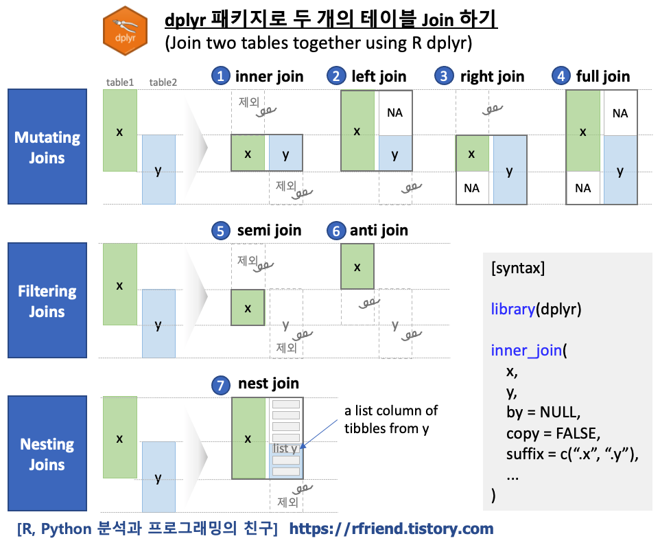
이번 포스팅에서는 dplyr 패키지를 사용하여 두 개의 지리공간 벡터 데이터 테이블을 Join 하는 여러가지 방법을 소개하겠습니다. [1] Database SQL에 이미 익숙한 분이라면 이번 포스팅은 매우 쉽습니다. 왜냐하면 dplyr 의 두 테이블 간 Join 이 SQL의 Join 을 차용해서 만들어졌기 때문입니다.
R의 sf 클래스 객체인 지리공간 벡터 데이터를 dplyr 의 함수를 사용해서 두 테이블을 join 하면 속성(attributes)과 함께 지리공간 geometry 칼럼과 정보도 join 된 후의 테이블에 자동으로 그대로 따라가게 됩니다.
(1) Mutating Joins : 두 테이블을 합쳐서 새로운 테이블을 생성하기
- (1-1) inner join
- (1-2) left join
- (1-3) right join
- (1-4) full join
(2) Filtering Joins : 두 테이블의 매칭되는 부분을 기준으로 한쪽 테이블을 걸러내기
- (2-1) semi join
- (2-2) anti join
(3) Nesting joins : 한 테이블의 모든 칼럼을 리스트로 중첩되게 묶어서 다른 테이블에 합치기
- (3-1) nest join
R dplyr 패키지가 두 테이블 Join 을 하는데 제공하는 함수는 inner_join(), left_join(), right_join(), full_join(), semi_join(), anti_join(), nest_join() 의 총 7개가 있으며, 이는 크게 (a) Mutating Joins, (b) Filtering Joins, (3) Nesting Joins의 3개의 범주로 분류할 수 있습니다.
[ R dplyr 패키지로 두 개의 테이블 Join 하기 (Joining two tables together using R dplyr) ]
joining two tables using R dplyr
(1) Mutating Joins
Mutation Joins 는 두 개의 테이블을 Key를 기준으로 Join 하여 두 개 테이블로 부터 가져온 (전체 또는 일부) 행과 모든 열로 Join 하여 새로운 테이블을 만들 때 사용합니다. 위의 그림에서 보는 바와 같이 왼쪽(Left Hand Side, LHS)의 테이블과 오른쪽(Right Hand Side, RHD)의 테이블로 부터 모두 행과 열을 가져와서 Join 된 테이블을 반환하며, 이때 왼쪽(LHS)와 오른쪽(RHS) 중에서 어느쪽 테이블이 기준이 되느냐에 따라 사용하는 함수가 달라집니다.
(1-1) inner join
먼저, 예제로 사용할 sf 클래스 객체로서, spData 패키지에서 세계 국가별 속성정보와 지리기하 정보를 가지고 있는 'world' 데이터셋, 그리고 2016년과 2017년도 국가별 커피 생산량을 집계한 coffee_data 데이터셋을 가져오겠습니다. "world" 데이터셋은 177개의 관측치, 11개의 칼럼을 가지고 있고, "coffee_data" 데이터셋은 47개의 관측치, 3개의 칼럼을 가지고 있습니다. 그리고 두 데이터셋은 공통적으로 'name_long' 이라는 국가이름 칼럼을 가지고 있으며, 이는 두 테이블을 Join 할 때 기준 Key 로 사용이 됩니다.
테이블 Join 을 위해 dplyr 패키지를 불러오겠습니다.
## ==================================
## GeoSpatial Data Analysis using R
## : Vector attribute joining
## : reference: https://geocompr.robinlovelace.net/attr.html
## ==================================

library(sf)
library(spData) # for sf data
library(dplyr)

## -- (a) world: World country pologons in spData
names(world)
# [1] "iso_a2"  "name_long" "continent" "region_un" "subregion" "type"  "area_km2"  "pop"  "lifeExp"   "gdpPercap"
# [11] "geom"

dim(world)
# [1] 177  11


## -- (b) coffee_data: World coffee productiond data in spData
## : estimated values for coffee production in units of 60-kg bags in each year
names(coffee_data)
# [1] "name_long"      "coffee_production_2016" "coffee_production_2017"

dim(coffee_data)
# [1] 47  3
dplyr 패키지의 테이블 Join 에 사용하는 함수들의 기본 구문은 아래와 같이 왼쪽(x, LHS), 오른쪽(y, RHS) 테이블, 두 테이블을 매칭하는 기준 칼럼(by), 데이터 source가 다를 경우 복사(copy) 여부, 접미사(suffix) 등의 매개변수로 구성되어 서로 비슷합니다.
## dplyr join syntax library(dplyr)
## -- (a) Mutating Joins inner_join(x, y, by = NULL, copy = FALSE, suffix = c(".x", ".y"), ...) left_join(x, y, by = NULL, copy = FALSE, suffix = c(".x", ".y"), ...) right_join(x, y, by = NULL, copy = FALSE, suffix = c(".x", ".y"), ...) full_join(x, y, by = NULL, copy = FALSE, suffix = c(".x", ".y"), ...)
## -- (b) Filtering Joins semi_join(x, y, by = NULL, copy = FALSE, ...) anti_join(x, y, by = NULL, copy = FALSE, ...)
## -- (c) Nesting Joins nest_join(x, y, by = NULL, copy = FALSE, keep = FALSE, name = NULL, ...)
inner join 은 두 테이블에서 Key 칼럼을 기준으로 서로 매칭이 되는 행에 대해서만, 두 테이블의 모든 칼럼을 반환합니다. 그럼, "world"와 "coffee_data" 두 데이터셋 테이블을 공통의 칼럼인 "name_long" 을 기준으로 inner join 해보겠습니다. 두 테이블에 공통으로 "name_long"이 존재하는 관측치가 45개가 있네요.
만약 두 테이블 x, y 에 다수의 매칭되는 값이 있을 경우에는, 모든 가능한 조합의 값을 반환하므로, 주의가 필요합니다.
dplyr 의 Join 함수들은 두 테이블 Join 의 기준이 되는 Key 칼럼 이름을 by 매개변수에 안써주면 두 테이블에 공통으로 존재하는 칼럼을 Key 로 삼아서 Join 을 수행하고, 콘솔 창에 'Joining, by = "name_long"' 과 같이 Key 를 출력해줍니다.
left join 은 왼쪽의 테이블(LHS, x)을 모두 반환하고 (기준이 됨), 오른쪽 테이블(RHS, y)은 왼쪽 테이블과 Key 값이 매칭되는 관측치에 대해서만 모든 칼럼을 왼쪽 테이블에 Join 하여 반환합니다. 만약 오른쪽 테이블(RHS, y)에 매칭되는 값이 없는 경우 x 테이블의 y에 해당하는 행은 NA 로 채워집니다.
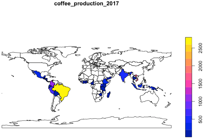
아래 예에서는 왼쪽에 있는 "world" 테이블을 기준으로 오른쪽의 "coffee_data"를 공통으로 존재하는 'name_long' 칼럼을 Key로 해서 left join 을 한 것입니다. 12번째와 13번째 칼럼에 오른쪽 테이블인 "coffee_data" 에서 Join 해서 가져온 "coffee_production_2016", "coffee_production_2017"의 칼럼이 왼쪽 "world" 테이블에 Join 이 되었습니다.
plot() 함수로 다면(multi-polygons) 기하도형으로 구성된 세계 국가별 지도에 2017년도 커피 생산량을 시각화해보았습니다. 지리기학 벡터 데이터를 Join 했을 때 누릴 수 있는 geometry 칼럼을 사용할 수 있는 혜택이 되겠습니다.
두 테이블을 Join 할 때 기준이 되는 Key 칼럼의 이름이 서로 다른 경우 by 매개변수에 서로 다른 변수 이름을 구체적으로 명시해주면 됩니다. 아래 예에서는 오른쪽 "coffee_data" 테이블의 'name_long' 칼럼 이름을 'nm'으로 바꿔준 후에, by = c(name_long = "nm") 처럼 Join하려는 두 테이블의 서로 다른 이름의 Key 변수들을 명시해주었습니다.
## -- Using the 'by' argument to specify the joining variables
coffee_renamed = rename(coffee_data, nm = name_long)
world_coffee2 = left_join(world, coffee_renamed,
                          by = c(name_long = "nm")) # specify the joining variables

names(world_coffee2)
# [1] "iso_a2"                 "name_long"              "continent"              "region_un"
# [5] "subregion"              "type"                   "area_km2"               "pop"
# [9] "lifeExp"                "gdpPercap"              "geom"                   "coffee_production_2016"
# [13] "coffee_production_2017"
(1-3) right join
right join 은 오른쪽 테이블(RHS, y) 을 전부 반환하고, 왼쪽 테이블 (LHS, x) 은 오른쪽(y) 테이블과 매칭이 되는 값에 대해서만 모든 칼럼을 Join 해서 반환합니다. Key 칼럼을 기준으로 왼쪽 테이블에 없는 값은 NA 처리가 되어 오른쪽 테이블에 Join 됩니다. (위의 그림 도식을 참고하세요).
만약 왼쪽과 오른쪽 테이블에 다수의 매칭되는 값들이 있을 경우 매칭되는 값들의 모든 조합으로 Join 됩니다. 아래 예에서 Join 의 기준이 되는 Key 를 명기해주는 매개변수 by = 'name_long' 는 두 테이블에 공통으로 존재하므로 생략 가능합니다.
## -- (1-3) right join: return all rows from y, and all columns from x.
world_coffee_right = right_join(x = world,
                                y = coffee_data,
                                by = 'name_long')


dim(world) # -- left
# [1] 177  11

dim(coffee_data) # -- right
# [1] 47  3

dim(world_coffee_right) # -- right join
# [1] 47 13
(1-4) full join
full Join 은 왼쪽 (LHS, x)과 오른쪽(RHS, y)의 모든 행과 열을 반환합니다.
## -- (1-4) full join: return all rows and all columns from both x and y.
world_coffee_full = full_join(x = world,
                              y = coffee_data,
                              by = 'name_long')

dim(world_coffee_full)
# [1] 179  13


names(world_coffee_full)
# [1] "iso_a2"        "name_long"   "continent"    "region_un"
# [5] "subregion"     "type"        "area_km2"     "pop"
# [9] "lifeExp"       "gdpPercap"   "geom"         "coffee_production_2016"
# [13] "coffee_production_2017"
어느 한쪽 테이블에서 버려지는 값이 없으며, 만약 왼쪽이나 오른쪽 테이블에 없는 값이면 "NA" 처리됩니다. 아래의 왼쪽 "world" 테이블과 오른쪽의 "coffee_data" 테이블 간에 서로 매칭되지 않는 부분은 "NA"가 들어가 있음을 알 수 있습니다.
## Where there are not matching values, returns 'NA' for the one missing.
head(world_coffee_full[, c(2:3, 9:13)], 10)

# Simple feature collection with 10 features and 6 fields
# geometry type:  MULTIPOLYGON
# dimension:      XY
# bbox:           xmin: -180 ymin: -55.25 xmax: 180 ymax: 83.23324
# geographic CRS: WGS 84
# # A tibble: 10 x 7
# name_long   continent   lifeExp gdpPercap                                        geom coffee_productio~ coffee_productio~
#   <chr>       <chr>         <dbl>     <dbl>                 <MULTIPOLYGON [arc_degree]>             <int>             <int>
#  1 Fiji        Oceania        70.0     8222. (((180 -16.06713, 180 -16.55522, 179.3641 ~                NA                NA
#  2 Tanzania    Africa         64.2     2402. (((33.90371 -0.95, 34.07262 -1.05982, 37.6~                81                66
#  3 Western Sa~ Africa         NA         NA  (((-8.66559 27.65643, -8.665124 27.58948, ~                NA                NA
#  4 Canada      North Amer~    82.0    43079. (((-122.84 49, -122.9742 49.00254, -124.91~                NA                NA
#  5 United Sta~ North Amer~    78.8    51922. (((-122.84 49, -120 49, -117.0312 49, -116~                NA                NA
#  6 Kazakhstan  Asia           71.6    23587. (((87.35997 49.21498, 86.59878 48.54918, 8~                NA                NA
#  7 Uzbekistan  Asia           71.0     5371. (((55.96819 41.30864, 55.92892 44.99586, 5~                NA                NA
#  8 Papua New ~ Oceania        65.2     3709. (((141.0002 -2.600151, 142.7352 -3.289153,~               114                74
#  9 Indonesia   Asia           68.9    10003. (((141.0002 -2.600151, 141.0171 -5.859022,~               742               360
# 10 Argentina   South Amer~    76.3    18798. (((-68.63401 -52.63637, -68.25 -53.1, -67.~                NA                N
(2) Filtering Joins
Filtering Joins 은 두 테이블의 매칭되는 값을 기준으로 한쪽 테이블의 값을 걸러내는데 사용합니다.
(2-1) semi join
semi join 은 왼쪽(LHS, x)과 오른쪽(RHS, y) 테이블의 서로 매칭되는 값에 대해 왼쪽(LHS, x)의 모든 칼럼을 반환합니다. 이때 매칭 여부를 평가하는데 사용되었던 오른쪽 테이블(RHS, y)의 값은 하나도 가져오지 않으며, 단지 왼쪽 테이블(x)을 걸러내느데(filtering)만 사용하였다는 점이 위의 (1-2) Left Join 과 다른 점입니다. (위의 도식을 참고하세요)
## -- (2) Filtering joins
## -- (2-1) semi join
## : return all rows from x where there are matching values in y,
## : keeping just columns form x.

world_coffee_semi = semi_join(world, coffee_data)
# Joining, by = "name_long"

dim(world_coffee_semi)
# [1] 45 11

names(world_coffee_semi)
# [1] "iso_a2"    "name_long" "continent" "region_un" "subregion" "type"  "area_km2"  "pop"
# [9] "lifeExp"   "gdpPercap" "geom"
(2-2) anti join
anti join 은 왼쪽 테이블(LHS, x)과 오른쪽 테이블(RHS, y)의 매칭되는 부분을 왼쪽 테이블(LHS, x)에서 걸러낸 x의 모든 칼럼을 반환합니다. 이때 매칭 여부를 평가하는데 사용되었던 오른쪽(RHS, y) 테이블의 값은 하나도 가져오지 않으며, 단지 왼쪽 테이블(x)을 걸러내는데(filtering)만 사용합니다.
위의 (2-1)의 semi join 은 x와 y의 매칭되는 부분의 x값만을 반환하였다면, 이번 (2-2)의 anti join 은 반대로 x와 j의 매칭이 안되는 부분의 x값만을 반환하는게 다릅니다. (y 값은 안가져오는 것은 semi join 과 anti join 이 동일함.)
## -- (6) anti join
## : return all rows from x where there are not matching values in y,
## : keeping just columns from x.
world_coffee_anti = anti_join(world, coffee_data)
# Joining, by = "name_long"

dim(world_coffee_anti)
# [1] 132  11

names(world_coffee_anti)
# [1] "iso_a2"    "name_long" "continent" "region_un" "subregion" "type"      "area_km2"  "pop"
# [9] "lifeExp"   "gdpPercap" "geom"
(3) Nesting Joins
(3-1) nest join
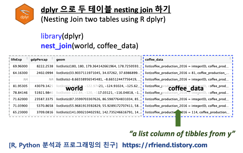
nest join 은 왼쪽 테이블(LHS, x)의 모든 행과 열을 반환하며, 이때 오른쪽(RHS, y)의 매칭되는 부분의 모든 칼럼의 값들을 list 형태로 중첩되게 묶어서 왼쪽 x 테이블에 join 해줍니다. 즉, 오른쪽 y 테이블의 매칭되는 값들의 칼럼이 여러개 이더라도 왼쪽 x 테이블에 join 이 될 때는 1개의 칼럼에 list 형태로 오른쪽 y 테이블의 여러개 칼럼의 값들이 묶여서 join 됩니다.
## -- (3) Nesting joins
## -- (3-1) nest join
## : eturn all rows and all columns from x. Adds a list column of tibbles.
## : Each tibble contains all the rows from y that match that row of x.
world_coffee_nest = nest_join(world, coffee_data)
# Joining, by = "name_long"

dim(world_coffee_nest)
# [1] 177  12

names(world_coffee_nest)
# [1] "iso_a2"      "name_long"   "continent"   "region_un"   "subregion"   "type"        "area_km2"
# [8] "pop"         "lifeExp"     "gdpPercap"   "geom"        "coffee_data"


head(world_coffee_nest[, 10:12], 3)
# Simple feature collection with 3 features and 2 fields
# geometry type:  MULTIPOLYGON
# dimension:      XY
# bbox:           xmin: -180 ymin: -18.28799 xmax: 180 ymax: 27.65643
# geographic CRS: WGS 84
# # A tibble: 3 x 3
# gdpPercap                                                                                geom coffee_data
# <dbl>                                                         <MULTIPOLYGON [arc_degree]> <list>
# 1     8222. (((180 -16.06713, 180 -16.55522, 179.3641 -16.80135, 178.7251 -17.01204, 178.5968 ~ <tibble [0 x 2~
# 2     2402. (((33.90371 -0.95, 34.07262 -1.05982, 37.69869 -3.09699, 37.7669 -3.67712, 39.2022~ <tibble [1 x 2~
# 3       NA  (((-8.66559 27.65643, -8.665124 27.58948, -8.6844 27.39574, -8.687294 25.88106, -1~ <tibble [0 x 2~
말로만 설명하면 잘 이해가 안될 듯 하여 아래에 nest_join(world, coffee_data) 된 테이블의 아웃풋을 화면 캡쳐하였습니다. nest join 된 후의 테이블에서 오른쪽의 "coffee_data" 라는 1개의 칼럼에 보면 list(coffee_proeuction_2016 = 81, coffee_proeuction_2017 = xx) 라고 해서 "coffee_data" 에 들어있는 2개의 칼럼이 1개의 리스트 형태의 칼럼에 중첩이 되어서 들어가 있음을 알 수 있습니다.
다음번 포스팅에서는 Join 했을 때 Join 의 기준이 되는 Key 값이 일부 표준화가 안되어서 제대로 Join 이 안될 경우에 정규 표현식(Regular expression)을 사용해서 Join 하는 방법(rfriend.tistory.com/626)을 소개하겠습니다.
지난번 포스팅에서는 지리공간 벡터 데이터의속성 정보의 행과 열을 가져오기 (rfriend.tistory.com/622) 에 대해서 알아보았습니다. 그리고 지리공간 벡터 데이터는 지리 정보(geometry column) + 속성 정보(attributes)로 이루어지며, 속성 정보의 일부를 subset 하여 가져오면 지리정보(geometry column)가 같이 따라 온다는 것도 소개하였습니다.
이번 포스팅에서는 지리공간 벡터 데이터의 속성 정보의 요약 정보를 그룹별로 집계하는 방법(aggregating geographic vector attritubes by group)을 R 패키지별로 나누어서 소개하겠습니다.
(1) Base R의 aggregate() 함수를 사용해서 지리 벡터 데이터의 속성 정보를 그룹별로 집계하기
(2) dplyr 의 summarise() 함수를 사용해서 지리 벡터 데이터의 속성 정보를 그룹별로 집계하기
(3) data.table 로 지리 벡터 데이터의 속성 정보를 그룹별로 집계하기
(1) Base R의 aggregate() 함수를 사용해서 지리 벡터 데이터의 속성 정보를 그룹별로 집계하기
그리고, Base R, dplyr, data.table 의 3개 패키지 내 함수를 사용해서 아래 문제의 그룹별 속성 정보 집계를 해보겠습니다.
대륙(continent) 그룹 별로 인구(pop) 속성 데이터의 합(summation)을 구하고, 국가의 수 (number of countries) 를 집계한 후, --> 인구 합이 가장 큰 상위 3개(top 3) 대륙을 선별하시오.
예제로 spData 패키지에 들어있는 'world' 라는 이름의, 10개 속성(attributes)과 1개 지리기하 칼럼(geometry column)을 가지고 있는 세계 국가에 대한 지리 벡터 데이터를 사용하겠습니다. 그리고 속성 정보 집계를 하는데 사용할 dplyr, data.table 패키지도 불러오겠습니다.
## =================================
## GeoSpatial Data Analysis using R
## : Vector attribute aggregation
## =================================

library(sf)
library(spData)     # for dataset
library(dplyr)      # for data aggregation
library(data.table) # for data aggregation

names(world)
# [1] "iso_a2"    "name_long" "continent" "region_un" "subregion" "type"      "area_km2"  "pop"       "lifeExp"   "gdpPercap"
# [11] "geom"
Base R 패키지에 기본으로 내장되어 있는 aggregate(x ~ group, FUN, data, ...) 함수를 사용해서 '대륙(continent)' 그룹별로 속성 정보인 '인구(pop)' 의 합(sum) 을 집계해보겠습니다. 이렇게 합계를 집계하면 data.frame 을 반환하였으며, 집계된 결과에 지리 기하(geometry) 정보는 없습니다.
## aggregation operations summarize dataset by a 'grouping variable'.

## (1) aggregation using aggregate() function from Base R
## : returns a non-spatial data.frame
world_agg_pop = aggregate(pop ~ continent,
                          FUN = sum,
                          data = world,
                          na.rm = TRUE)

str(world_agg_pop)
# 'data.frame':	6 obs. of  2 variables:
#   $ continent: chr  "Africa" "Asia" "Europe" "North America" ...
# $ pop      : num  1.15e+09 4.31e+09 6.69e+08 5.65e+08 3.78e+07 ...

class(world_agg_pop)
# [1] "data.frame"


world_agg_pop
# continent        pop
# 1        Africa 1154946633
# 2          Asia 4311408059
# 3        Europe  669036256
# 4 North America  565028684
# 5       Oceania   37757833
# 6 South America  412060811
'sf' 객체에 대해 aggregate() 함수를 적용하면 'sf' 클래스에 있는 aggregate.sf() 함수가 자동으로 활성화되어 적용이 됩니다. world['pop'] 의 'sf' 클래스를 x 로 하여 aggregate(x = sf_object, by = list(), FUN, ...) 구문으로 아래와 같이 대륙 그룹별로 인구의 합계를 집계하면"data.frame"을 확장한 "sf" 클래스의 집계된 객체를 반환하며, "data.frame"의 제일 끝에 "geometry" 칼럼이 리스트로 같이 집계(aggregation)가 됩니다. (즉, 각 대륙별로 국가들의 다각형 면(polygon)을 모아놓은 리스트가 "geometry"에 생김).
## aggregate.sf() is activated automatically when 'x' is an sf object and a 'by' argument is provided.
## : returns a spatial 'sf' class and data.frame
world_agg_pop2 = aggregate(
  x = world['pop'],
  by = list(world$continent), # a lost of grouping elements
  FUN = sum,
  na.rm = TRUE)

str(world_agg_pop2)
# Classes 'sf' and 'data.frame':	8 obs. of  3 variables:
#   $ Group.1 : chr  "Africa" "Antarctica" "Asia" "Europe" ...
# $ pop     : num  1.15e+09 0.00 4.31e+09 6.69e+08 5.65e+08 ...
# $ geometry:sfc_GEOMETRY of length 8; first list element: List of 2
# ..$ :List of 1
# .. ..$ : num [1:356, 1:2] 32.8 32.6 32.5 32.2 31.5 ...
# ..$ :List of 1
# .. ..$ : num [1:49, 1:2] 49.5 49.8 50.1 50.2 50.5 ...
# ..- attr(*, "class")= chr [1:3] "XY" "MULTIPOLYGON" "sfg"
# - attr(*, "sf_column")= chr "geometry"
# - attr(*, "agr")= Factor w/ 3 levels "constant","aggregate",..: 3 2
# ..- attr(*, "names")= chr [1:2] "Group.1" "pop"


class(world_agg_pop2)
# [1] "sf"         "data.frame"

names(world_agg_pop2)
# [1] "Group.1"  "pop"      "geometry"

world_agg_pop2
# Simple feature collection with 8 features and 2 fields
# Attribute-geometry relationship: 0 constant, 1 aggregate, 1 identity
# geometry type:  GEOMETRY
# dimension:      XY
# bbox:           xmin: -180 ymin: -90 xmax: 180 ymax: 83.64513
# geographic CRS: WGS 84
# Group.1        pop                       geometry
# 1                  Africa 1154946633 MULTIPOLYGON (((32.83012 -2...
# 2              Antarctica          0 MULTIPOLYGON (((-163.7129 -...
# 3                    Asia 4311408059 MULTIPOLYGON (((120.295 -10...
# 4                  Europe  669036256 MULTIPOLYGON (((-51.6578 4....
# 5           North America  565028684 MULTIPOLYGON (((-61.68 10.7...
# 6                 Oceania   37757833 MULTIPOLYGON (((169.6678 -4...
# 7 Seven seas (open ocean)          0 POLYGON ((68.935 -48.625, 6...
# 8           South America  412060811 MULTIPOLYGON (((-66.95992 -...
참고로, world['pop'] 는 "sf" 객체이기 때문에 aggregate() 함수 적용 시 자동으로 ''sf" 클래스의 aggregate.sf() 함수가 자동으로 활성화되어 적용되고 집계 결과가 "sf" 객체로 반환되는 반면에, world$pop 는 숫자형 벡터(numeric vector) 이므로 aggregate() 함수를 적용하면 "data.frame" 으로 집계 결과를 반환하게 됩니다.
이제 우리가 풀고자 하는 요구사항에 답해보겠습니다. 요구사항은 "대륙 그룹별로 속성정보인 인구(pop)의 합과 국가의 수를 집계하고, 인구 합을 기준으로 상위 3개의 대륙을 찾으라"는 것이었습니다. aggregate(x ~ group, data, FUN) 구문으로 그룹별 집계를 하되, 집계해야 할 것이 (a) 인구의 "합(sum)"과, & (b) 국가의 "개수(number of rows)" 의 2개 이므로 FUN = function(x) c(pop = sum(x), n = length(x)) 의 함수를 사용해서 합과 개수를 구하도록 했습니다. 그리고 do.call(data.frame, ...) 을 사용해서 리스트로 반환된 집계 결과를 data.frame으로 변환을 해주었습니다.
그리고 "인구 합을 기준으로 상위 3개 대륙"을 찾기 위해서 order(-world_pop$pop.pop) 로 내림차순 정렬('-' 부호가 내림차순 정렬을 의미함. order 는 정렬 후의 위치 인덱스를 반환함.)을 한 인덱스를 사용해서 정렬을 한 후에 [1:3, ] 으로 상위 3개 행만을 가져왔습니다.
## group by aggregation: sum of pop, number of rows
world_pop = do.call(data.frame, aggregate(pop ~ continent,
                      data = world,
                      FUN = function(x) c(pop = sum(x), n = length(x))))


## sorting by pop.pop in descending order and select top 3
world_pop[order(-world_pop$pop.pop),][1:3,]

#   continent    pop.pop pop.n
# 2      Asia 4311408059    45
# 1    Africa 1154946633    48
# 3    Europe  669036256    37
(2) dplyr 의 summarise() 함수를 사용해서 지리 벡터 데이터의 속성 정보를 그룹별로 집계하기
위의 (1)번에서는 Base R의 aggregate() 함수를 사용하였는데요, dplyr 패키지의 group_by() 로 기준이 되는 그룹을 지정해주고 summarise() (또는 summarize()) 함수를 사용해서 다양한 집계 함수를 사용하여 Base R 보다 가독성이 좋고 속도가 빠른 코드를 짤 수 있습니다.
아래는 dplyr 패키지의 체인(%>%) 으로 파이프 연산자(pipe operator)를 사용해서 대륙 그룹별로 인구의 합계를 구해본 것입니다. 이때, 'sf' 객체에 대해 summarise() 함수를 적용하면 집계 결과는 자동으로 "data.frame"을 확장한 "sf" 클래스의 객체로 반환을 하고, 제일 마지막 칼럼에 "geom" 지리기하 리스트를 포함하게 됩니다.
## (2) aggregation using summarise() function from dplyr
library(dplyr)

world_agg_pop3 = world %>%
  group_by(continent) %>%
  summarise(sum(pop, na.rm = TRUE))

class(world_agg_pop3)
# [1] "sf"         "tbl_df"     "tbl"        "data.frame"

names(world_agg_pop3)
# [1] "continent" "pop"   "geom"
dplyr 의 summarise() 함수를 쓰면 (a) 집계한 결과의 칼럼 이름을 새로 부여할 수 있고, (b) 여러개의 집계 함수(예: 합, 개수, 평균, 표준편차, 최대, 최소 등)를 동시에 사용할 수 있다는 편리한 장점이 있습니다.
아래 예에서는 대륙별로 인구에 대한 합(sum(pop, na.rm=TRUE))과 국가의 개수(n()) 를 구하고, 집계된 후 결과의 칼럼 이름도 "pop_sum", "n_countries" 로 새로 부여해 본 것입니다.
이제 위에서 주어진 요구사항인 "대륙 그룹별로 인구의 합계와 국가 수를 집계하고, 인구합을 기준으로 상위 3개 대륙을 찾으라"는 문제를 dplyr 의 체인 파이프 연산자를 써서 풀어보겠습니다. top_n(n = 3, wt = pop) 함수로 인구합을 기준으로 상위 3개를 구하였고, arrange(desc(pop)) 로 인구합을 기준으로 내림차순 정렬하였습니다. 이때 지리기하 칼럼은 생략하고 속성(attritubes)에 대한 집계 결과만 얻고자 하므로 제일 마지막에 st_drop_geometry() 함수로 "geometry" 칼럼을 제거하였습니다.
## finding the world's 3 most populous continents by chaining functions using dplyr
world %>%
  dplyr::select(pop, continent) %>%
  group_by(continent) %>%
  summarise(pop = sum(pop, na.rm = TRUE), n_countries = n()) %>%
  top_n(n = 3, wt = pop) %>% # select top 3 rows by 'pop' varialbe
  arrange(desc(pop)) %>%     # sorting in a descending order
  st_drop_geometry()         # drop geometry column

# `summarise()` ungrouping output (override with `.groups` argument)
# # A tibble: 3 x 3
# continent        pop n_countries
# * <chr>          <dbl>       <int>
#   1 Asia      4311408059          47
# 2 Africa    1154946633          51
# 3 Europe     669036256          39
(3) data.table 로 지리 벡터 데이터의 속성 정보를 그룹별로 집계하기
마지막으로 data.table 패키지를 사용해서 "대륙 그룹별로 인구 합계와 국가 수를 집계하고, 인구 합계 기준 상위 3개 대륙을 찾으라"는 문제를 풀어보겠습니다.
먼저, world_dt = data.table(world) 로 'world' sf 객체를 data.table 객체로 변환하였습니다. 그리고 data.table 의 체인 파이프를 사용해서 필요한 작업 흐름을 이어서 작성해보았는데요, 역시 data.table 이 코드가 가장 간결하고, 또 속도도 가장 빠릅니다. 아래 코드에서 .(pop = sum(pop, na.rm = T), n = .N) 은 인구 합계(sum(pop, na.rm=T)와 행의 개수(.N) 를 대륙 그룹별로(by = list(continent)) 집계한 후에, [order(-pop)] 로 인구 합계를 기준으로 내림차순 정렬('-' 부호는 내림차순을 의미함)을 하고, [1:3]으로 상위 3개 대륙의 집계 결과만 가져온 것입니다. 코드가 '간결함' 그 자체입니다!
단, 이때 최종 집계 결과는 data.table 로 반환이 되며, 지리기하 정보는 없습니다.
## (3) aggregating vector attributes using data.table package
library(data.table)

world_dt = data.table(world)

world_dt[, .(pop = sum(pop, na.rm = TRUE), n = .N),
         by = list(continent)][order(-pop)][1:3]

## or equivalently above, using chaining
world_dt[,
         .(pop = sum(pop, na.rm = TRUE), n = .N), # aggregate
         by = list(continent)][    # by groups
           order(-pop)][           # sorting in descending order
             1:3]                  # subset rows (1:3)

# continent        pop  n
# 1:      Asia 4311408059 47
# 2:    Africa 1154946633 51
# 3:    Europe  669036256 39
만약, 그룹별 지리기하 벡터 데이터를 집계한 결과에 지리기하 칼럼(geometry column)을 같이 리스트로 묶어서 속성정보와 함께 집계하고 싶으면 data.table 객체에서 칼럼을 가져올 때 world_dt[, .(pop = sum(pop, na.rm = T), n = .N, geom = geom) 처럼 "geom" 칼럼도 같이 가져오고, 이후의 집계 및 정렬, 인덱싱은 동일합니다.
## with geometry column (lists)
world_dt[, .(pop = sum(pop, na.rm = TRUE), n = .N, geom = geom),
         by = list(continent)][order(-pop)][1:3]
# continent        pop  n     geom
# 1:      Asia 4311408059 47  <XY[1]>
# 2:      Asia 4311408059 47  <XY[1]>
# 3:      Asia 4311408059 47 <XY[13]>
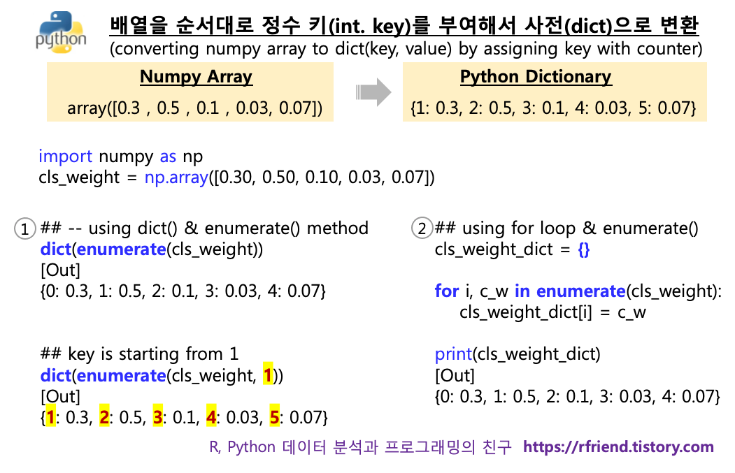
위의 'cls_weight' 배열을 사전(dictionary)으로 변환해보겠습니다. 사전(dict) 키(Key)가 '0' 부터 시작하고, 배열의 순서대로 사전의 키가 하나씩 증가하며, 배열의 순서대로 사전에 값을 할당하여 보겠습니다. dict() 함수는 객체를 '키(Key) : 값(Value)' 의 쌍을 가지는 사전형 자료구조를 만들어줍니다.
## converting numpy array to dictionary,
## dict key is starting from 0
cls_weight_dict_from_0 = dict(enumerate(cls_weight))

cls_weight_dict_from_0
[Out]
{0: 0.3, 1: 0.5, 2: 0.1, 3: 0.03, 4: 0.07}
이때 dict() 안의 enumerate() 메소드는 객체를 순환할 때 회수를 세어주는 counter 를 같이 생성해서 enumerate 객체를 반환합니다. for loop 으로 enumerate 객체를 순환하면서 counter 와 배열 내 값을 차례대로 출력을 해보면 아래와 같습니다.
## enumerate() method adds a counter to an iterable
## and returns it in a form of enumerate object
for i, j in enumerate(cls_weight):
    print(i, ':', j)

[Out]
0 : 0.3
1 : 0.5
2 : 0.1
3 : 0.03
4 : 0.07
경우에 따라서는 배열의 값으로 사전을 만들었을 때, 사전의 키 값이 '0'이 아니라 '1'이나 혹은 다른 숫자로 부터 시작하는 것을 원할 수도 있습니다. 이럴 경우 enumerate(iterable_object, 1) 처럼 원하는 숫자(아래 예에서는 '1')를 추가해주면 그 값이 더해져서 counter 가 생성이 됩니다.
## converting numpy array to dictionary,
## dict key is starting from 1

cls_weight_dict_from_1 = dict(enumerate(cls_weight, 1))

cls_weight_dict_from_1
[Out]
{1: 0.3, 2: 0.5, 3: 0.1, 4: 0.03, 5: 0.07}
만약 사전(dictionary)으로 변환하려고 하는 numpy array의 axis 1의 축이 있다면 flatten() 메소드를 사용해서 axis 0 만 있는 배열로 먼저 평평하게 펴준 (axis 1 축을 없앰) 후에 위의 dict(enumerate()) 를 똑같이 사용해주면 됩니다. 아래 예는 shape (5, 1) 의 배열을 flatten() 메소드를 써서 shape (5, 0) 으로 바꿔준 후에 dict(enumerate()) 로 배열을 사전으로 변환해주었습니다.
이번에는 for loop 과 enumerate() 메소드를 같이 이용하는 방법입니다. 위의 (1) 번 대비 좀 복잡한 느낌이 있기는 하지만, (1) 번 대비 (2) 방법은 for loop 안의 코드 블럭에 좀더 자유롭게 원하는 복잡한 로직을 녹여서 사전(dictionary)을 구성할 수 있다는 장점이 있습니다.
아래 예에서는 (a) 먼저 cls_weight_dict_3 = {} 로 비어있는 사전을 만들어 놓고, (b) for loop 으로 순환 반복을 하면서 enumerate(cls_weight) 가 반환해주는 (counter, 배열값) 로 부터 counter 정수 숫자를 받아서 cls_weight_dict_3 의 키(Key) 로 할당해주고, 배열의 값을 사전의 해당 키에 할당해주는 방식입니다. 사전의 키에 값 할당(assinging Value to dict by mapping Key)은 Dict[Key] = Value 구문으로 해줍니다.
cls_weight = np.array([0.30, 0.50, 0.10, 0.03, 0.07])
cls_weight
[Out]
array([0.3 , 0.5 , 0.1 , 0.03, 0.07])

## Converting a numpy array to a dictionary
## Dict key is starting from 0
cls_weight_dict_3 = {}

for i, c_w in enumerate(cls_weight):
    cls_weight_dict_3[i] = c_w


print(cls_weight_dict_3)
[Out]
{0: 0.3, 1: 0.5, 2: 0.1, 3: 0.03, 4: 0.07}
사전의 키를 '0' 이 아니라 '1'부터 시작하게 하려면 enumerate()의 counter가 0부터 시작하므로, counter를 사전의 키에 할당할 때 'counter+1' 을 해주면 됩니다.
## converting a numpy array to a dictionary using for loop
## dict key is strating from 1

## null dict
cls_weight_dict_3_from_1 = {}

## assigning values by keys + 1
for i, c_w in enumerate(cls_weight):
    cls_weight_dict_3_from_1[i+1] = c_w


print(cls_weight_dict_3_from_1)
[Out]
{1: 0.3, 2: 0.5, 3: 0.1, 4: 0.03, 5: 0.07}
Tistory 의 코드 블록에 'R' 언어도 사용할 수 있게 해달라고 며칠전에 제안 문의를 드렸었는데요, 드디어 'R' 언어가 추가되었네요. 잘 사용하겠습니다. Tistory, 감사합니다. 꾸벅~!
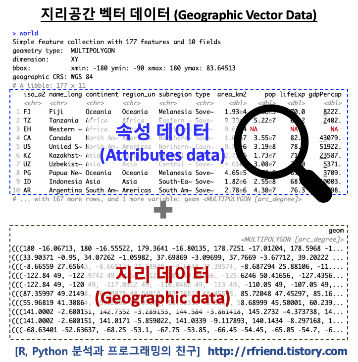
지리공간 벡터 데이터는 (a) 점(point), 선(linestring), 면(polygon) 등의 리스트로 이루어진 지리공간 데이터(geographic data)와, 지리공간 데이터를 제외한 (b) 속성 데이터(attribute data)로 구성이 됩니다. 속성 데이터(attritubes)를 사용해서 각 지리공간 별 특성 (예: 지역 이름, 면적, 인구, 예상수명 등)을 표현하게 됩니다.
이번 포스팅에서는 벡터 데이터에서 속성 정보를 가져오는 여러가지 방법을 소개하겠습니다. 'sf' 객체는 R data.frame 에서 사용하는 클래스를 지원(!!!)하므로 Base R 이나 혹은 dplyr 패키지를 사용하여 데이터 전처리하는 작업에 이미 능숙한 분이라면 이번 포스팅은 특별한 것 없이 매우 쉽게, 복습하는 기분으로 보실 수 있을 거예요.
(1) 'sf' 객체에서 속성 정보만 가져오기: st_drop_geometry()
(2) Base R 구문으로 벡터 데이터 속성 정보의 행과 열 가져오기 (subsetting attributes from geographic vector data using Base R)
(3) dplyr 로 벡터 데이터 속성 정보의 행과 열 가져오기 (subsetting attributes from geographic vector data using dplyr)
(4) 한개 칼럼만 가져온 결과를 벡터로 반환하기 (extracting a single vector)
먼저, 지리공간 데이터 객체를 다루기 위한 sf 패키지와 데이터 전처리에 사용할 dplyr 패키지를 불러오고, 예제로 사용할 세계 나라 데이터 ('world') 를 spData 패키지로 부터 가져오겠습니다.
'world' 벡터 데이터셋은 10개의 속성 데이터 (10 attributes) 와 1개의 지리기하 칼럼 (1 geometry column) 으로 구성이 되어 있으며, 총 177개의 행 (즉, 국가) 에 대한 정보가 들어 있습니다.
## ==============================
## R GeoSpatial data analysis
## - Vector Attribute data operations
## - reference: https://geocompr.robinlovelace.net/attr.html
## ==============================

library(sf)
library(dplyr)
library(spData)

## vector dataset 'world': 10 attritubes and 1 geometry column
str(world)
# tibble [177 x 11] (S3: sf/tbl_df/tbl/data.frame)
# $ iso_a2   : chr [1:177] "FJ" "TZ" "EH" "CA" ...
# $ name_long: chr [1:177] "Fiji" "Tanzania" "Western Sahara" "Canada" ...
# $ continent: chr [1:177] "Oceania" "Africa" "Africa" "North America" ...
# $ region_un: chr [1:177] "Oceania" "Africa" "Africa" "Americas" ...
# $ subregion: chr [1:177] "Melanesia" "Eastern Africa" "Northern Africa" "Northern America" ...
# $ type     : chr [1:177] "Sovereign country" "Sovereign country" "Indeterminate" "Sovereign country" ...
# $ area_km2 : num [1:177] 19290 932746 96271 10036043 9510744 ...
# $ pop      : num [1:177] 8.86e+05 5.22e+07 NA 3.55e+07 3.19e+08 ...
# $ lifeExp  : num [1:177] 70 64.2 NA 82 78.8 ...
# $ gdpPercap: num [1:177] 8222 2402 NA 43079 51922 ...
# $ geom     :sfc_MULTIPOLYGON of length 177; first list element: List of 3
# ..$ :List of 1
# .. ..$ : num [1:8, 1:2] 180 180 179 179 179 ...
# ..$ :List of 1
# .. ..$ : num [1:9, 1:2] 178 178 179 179 178 ...
# ..$ :List of 1
# .. ..$ : num [1:5, 1:2] -180 -180 -180 -180 -180 ...
# ..- attr(*, "class")= chr [1:3] "XY" "MULTIPOLYGON" "sfg"
# - attr(*, "sf_column")= chr "geom"
# - attr(*, "agr")= Factor w/ 3 levels "constant","aggregate",..: NA NA NA NA NA NA NA NA NA NA
# ..- attr(*, "names")= chr [1:10] "iso_a2" "name_long" "continent" "region_un" ...

dim(world)
# [1] 177  11
(1) 'sf' 객체에서 속성 정보만 가져오기: st_drop_geometry()
지리공간 'sf' 객체에는 항상 점(points)/선(lines)/면(polygons) 등의 지리기하 데이터를 리스트로 가지고 있는 geometry 칼럼이 항상 따라 다닙니다. 만약 'sf' 객체로 부터 이 geometry 칼럼을 제거하고 나머지 속성 정보만으로 DataFrame 을 만들고 싶다면 sf 패키지의 st_drop_geometry() 메소드를 사용합니다. geometry 칼럼의 경우 지리기하 점/선/면 등의 리스트 정보를 가지고 있기 때문에 메모리 점유가 크기 때문에, 사용할 필요가 없다면 geometry 칼럼은 제거하고 속성 정보만 dataframe 으로 만들어서 분석을 진행하는게 좋겠습니다.
(아래의 (2)번 부터 소개하는 부분 가져오기(subset) 방법을 사용하면 여전히 geometry 칼럼이 그림자차럼 같이 따라와서 여전히 달라붙어 있을 것입니다.)
## Extracting the attribute data of an 'sf' object
world_df <- st_drop_geometry(world)
class(world_df)
# [1] "tbl_df"     "tbl"        "data.frame"

names(world_df)
# [1] "iso_a2"    "name_long" "continent" "region_un" "subregion" "type"      "area_km2"  "pop"
# [9] "lifeExp"  "gdpPercap
(2) Base R 구문으로 벡터 데이터 속성 정보의 행과 열 가져오기 (subsetting attributes from geographic vector data using Base R)
R data.frame 에서 i 행(row)과 j 열(column)을 가져올 때는 df[i, j] , subset(), $ 구문을 사용합니다. 이때 (a) i 행과 j 열에는 정수로 위치(subset rows and columns by position) 을 사용하거나, (b) j 행의 이름 (subset columns by name)을 사용할 수 있으며, (c) 논리 벡터 (logical vector)를 사용해서 i 행의 부분집합(subset rows by a logical vector) 을 가져올 수 있습니다.
여기서 다시 한번 짚고 넘어갈 점은, 특정 행과 열의 부분집합을 가져오면 제일 끝에 geometry 칼럼이 꼭 껌딱지처럼 달라붙어서 같이 따라온다는 점입니다.
(2-a-1) 위치를 지정해서 지리공간 벡터 데이터로 부터 부분 행 가져오기 (subset rows by position)
## -- Vecter arrtibute subsetting
## subsetting columns returns results with geometry column as well.

## -- subset rows by position
world[1:3, ]

# Simple feature collection with 6 features and 10 fields
# geometry type:  MULTIPOLYGON
# dimension:      XY
# bbox:           xmin: -180 ymin: -18.28799 xmax: 180 ymax: 83.23324
# geographic CRS: WGS 84
# # A tibble: 6 x 11
# iso_a2 name_long  continent  region_un subregion type   area_km2     pop lifeExp gdpPercap                           geom
# <chr>  <chr>      <chr>      <chr>     <chr>     <chr>     <dbl>   <dbl>   <dbl>     <dbl>    <MULTIPOLYGON [arc_degree]>
#   1 FJ     Fiji       Oceania    Oceania   Melanesia Sover~   1.93e4  8.86e5    70.0     8222. (((180 -16.06713, 180 -16.555~
#   2 TZ     Tanzania   Africa     Africa    Eastern ~ Sover~   9.33e5  5.22e7    64.2     2402. (((33.90371 -0.95, 34.07262 -~
#   3 EH     Western S~ Africa     Africa    Northern~ Indet~   9.63e4 NA         NA         NA  (((-8.66559 27.65643, -8.6651~
(2-a-2) 위치를 지정해서 지리공간 벡터 데이터로 부터 부분 열 가져오기 (subset columns by position)
## -- subset columns by position
world[, 1:3]

# Simple feature collection with 177 features and 3 fields
# geometry type:  MULTIPOLYGON
# dimension:      XY
# bbox:           xmin: -180 ymin: -90 xmax: 180 ymax: 83.64513
# geographic CRS: WGS 84
# # A tibble: 177 x 4
# iso_a2 name_long        continent                                                                                   geom
# <chr>  <chr>            <chr>                                                                <MULTIPOLYGON [arc_degree]>
# 1 FJ     Fiji             Oceania       (((180 -16.06713, 180 -16.55522, 179.3641 -16.80135, 178.7251 -17.01204, 178.5968~
# 2 TZ     Tanzania         Africa        (((33.90371 -0.95, 34.07262 -1.05982, 37.69869 -3.09699, 37.7669 -3.67712, 39.202~
# 3 EH     Western Sahara   Africa        (((-8.66559 27.65643, -8.665124 27.58948, -8.6844 27.39574, -8.687294 25.88106, -~
# 4 CA     Canada           North America (((-122.84 49, -122.9742 49.00254, -124.9102 49.98456, -125.6246 50.41656, -127.4~
# 5 US     United States    North America (((-122.84 49, -120 49, -117.0312 49, -116.0482 49, -113 49, -110.05 49, -107.05 ~
# 6 KZ     Kazakhstan       Asia          (((87.35997 49.21498, 86.59878 48.54918, 85.76823 48.45575, 85.72048 47.45297, 85~
# 7 UZ     Uzbekistan       Asia          (((55.96819 41.30864, 55.92892 44.99586, 58.50313 45.5868, 58.68999 45.50001, 60.~
# 8 PG     Papua New Guinea Oceania       (((141.0002 -2.600151, 142.7352 -3.289153, 144.584 -3.861418, 145.2732 -4.373738,~
# 9 ID     Indonesia        Asia          (((141.0002 -2.600151, 141.0171 -5.859022, 141.0339 -9.117893, 140.1434 -8.297168~
# 10 AR     Argentina        South America (((-68.63401 -52.63637, -68.25 -53.1, -67.75 -53.85, -66.45 -54.45, -65.05 -54.7,~
# # ... with 167 more rows
(2-b) 칼럼 이름을 사용해서 지리공간 벡터 데이터로 부터 부분 열 가져오기 (subset columns by name)
(2-c) 논리 벡터를 사용해서 지리공간 벡터 데이터로 부터 부분 행 가져오기 (subset rows by a logical vectors)
## -- subset using 'logical vectors'
small_area_bool <- world$area_km2 < 10000
summary(small_area_bool)
#    Mode   FALSE    TRUE
# logical     170       7

small_countries <- world[small_area_bool, ]
nrow(small_countries)
# [1]  7

## or equivalently above
small_countries <- world[world$area_km2 < 10000, ]

## -- using base R subset() function
small_countries <- subset(world, area_km2 < 10000)
(3) dplyr 로 벡터 데이터 속성 정보의 행과 열 가져오기 (subsetting attributes from geographic vector data using dplyr)
R의 dplyr 패키지를 사용해서 지리공간 벡터 데이터의 속성 정보를 처리하면 Base R 대비 코드의 가독성이 좋고, 속도가 빠르다는 장점이 있습니다. dplyr 패키지에서 체인('%>%')으로 파이프 연산자 (pipe operator) 를 사용하면 작업 흐름 (work flow) 를 자연스럽게 따라가면서 코딩을 할 수 있어서 코드의 가독성이 상당히 좋습니다. 그리고 dplyr 은 소스코드가 C++로 되어 있어 속도도 상당히 빠른 편입니다.
dplyr 의 select(), slice(), filter(), pull() 함수를 사용해서 지리공간 벡터 데이터의 속성 정보의 부분 행과 열을 가져와 보겠습니다.
(3-1) dplyr::select(sf, name) 함수를 사용하여 이름으로 특정 열 선택하기 (selects columns by name)
이때, select() 함수는 dplyr 패키지 뿐만 아니라 raster 패키지에도 존재하므로 dplyr::select() 처럼 select() 함수 이름 앞에 패키지 이름을 명시적으로 같이 표기해 줌으로써 불명확성을 없앨 수 있습니다. dplyr::select(data.frame 이름, 칼럼1, 칼럼2, ...) 의 구문으로 원하는 열의 속성 정보만 가져올 수 있습니다. (지리공간 벡터 데이터라고 해서 select() 구문에는 특별한 것이 없으며, subset 결과의 끝에 geometry 칼럼이 달라 붙어서 따라와 있다는 점이 다릅니다.)
(3-2) dplyr::select(sf, position) 함수를 사용하여 위치로 특정 열 선택하기 (select columns by position)
## select() columns by position
world1 = dplyr::select(world, 2, 7)

names(world1)
# [1] "name_long" "area_km2"  "geom"
(3-3) dplyr::select(sf, name1:name2) 함수를 사용하여 범위 내의 모든 열 선택하기 (a range of columns by ':')
':' 연산자를 사용하여 두개의 위치(position1:position2)나 칼럼 이름(name1:name2)들의 범위 사이에 들어있는 모든 열을 한꺼번에 가져올 수 있습니다. 선택해서 가져오고 싶은 열이 많고 범위로 표현할 수 있을 경우 유용합니다.
## select() also allows subsetting of a range of columns with the help of the : operator
world2 = dplyr::select(world, name_long:area_km2)

names(world2)
# [1] "name_long" "continent" "region_un" "subregion" "type"   "area_km2"  "geom"
(3-4) dplyr::select(sf, -name) 으로 특정 열을 제거하기 (omit specific columns with the - operator)
## Omit specific columns with the - operator
# all columns except subregion and area_km2 (inclusive)
world3 = dplyr::select(world, -region_un, -subregion, -area_km2, -gdpPercap)

names(world3)
# [1] "iso_a2"    "name_long" "continent" "type"      "pop"       "lifeExp"   "geom"
(3-5) dplyr::select(sf, name_new = name_old) 로 선택해서 가져온 열 이름을 바꾸기 (subset & rename columns)
## select() lets you subset and rename columns at the same time
world4 = dplyr::select(world, name_long, population = pop)

names(world4)
# [1] "name_long"  "population" "geom"
(3-6) dplyr::select(sf, contains(string)) 로 특정 문자열을 포함한 칼럼을 선택하기
dplyr 의 select() 함수는 contains(), starts_with(), ends_with(), num_range() 와 같은 도우미 함수 (helper functions) 를 사용해서 매우 강력하고 편리하게 특정 칼럼을 선택해서 가져올 수 있습니다.
## select() works with ‘helper functions’ for advanced subsetting operations,
## including contains(), starts_with() and num_range()
## contains(): Contains a literal string
world5 = dplyr::select(world, contains('Ex'))

names(world5)
# [1] "lifeExp" "geom"
(3-7) dplyr::select(sf, starts_with(string)) 로 특정 문자열로 시작하는 칼럼을 선택하기
## starts_with(): Starts with a prefix
world6 = dplyr::select(world, starts_with('life'))

names(world6)
# [1] "lifeExp" "geom"
(3-8) dplyr::select(sf, ends_with(string)) 로 특정 문자열로 끝나는 칼럼을 선택하기
## ends_with(): Ends with a suffix
world7 = dplyr::select(world, ends_with('Exp'))

names(world7)
# [1] "lifeExp" "geom"
(3-9) dplyr::select(df, matches(regular_expression)) 으로 정규 표현식을 만족하는 특정 칼럼을 선택하기
아래 예는 정규 표현식(regular expression) "[p]" 를 matches() 도움미 함수 안에 사용해서, 칼럼 이름에 대/소문자 'p' 문자열이 들어있는 칼럼을 선택해서 가져온 것입니다.
(3-10) dplyr::select(df, num_range("x", num1:num2)) 으로 숫자 범위 안의 모든 칼럼 선택하기
만약 칼럼 이름이 "x1", "x2", "x3", "x4", "x5" 처럼 접두사(prefix)가 동일하고 뒤에 순차적인 정수가 붙어있는 형태라면 특정 정수 범위의 칼럼들을 선택해서 가져올 때 num_range() 도우미 함수를 select() 함수 안에 사용할 수 있습니다. "world" sf 객체의 데이터셋은 칼럼 이름이 특정 접두사로 동일하게 시작하지 않으므로, 아래에는 간단한 data.frame 을 만들어서 예를 들어보였습니다.
(3-11) dplyr::slice(sf, position1:position2) 으로 특정 행 잘라서 가져오기 (slice rows by position)
## -- slice(): is the row-equivalent of select()
dplyr::slice(world, 3:5)

# Simple feature collection with 3 features and 10 fields
# geometry type:  MULTIPOLYGON
# dimension:      XY
# bbox:           xmin: -171.7911 ymin: 18.91619 xmax: -8.665124 ymax: 83.23324
# geographic CRS: WGS 84
# # A tibble: 3 x 11
# iso_a2 name_long continent region_un subregion type  area_km2     pop lifeExp gdpPercap
# <chr>  <chr>     <chr>     <chr>     <chr>     <chr>    <dbl>   <dbl>   <dbl>     <dbl>
#   1 EH     Western ~ Africa    Africa    Northern~ Inde~   9.63e4 NA         NA         NA
# 2 CA     Canada    North Am~ Americas  Northern~ Sove~   1.00e7  3.55e7    82.0    43079.
# 3 US     United S~ North Am~ Americas  Northern~ Coun~   9.51e6  3.19e8    78.8    51922.
# # ... with 1 more variable: geom <MULTIPOLYGON [arc_degree]>
(3-12) dplyr::filter(sf, logical_vector) 로 조건을 만족하는 특정 행 걸러내기 (filter rows with conditions)
## -- filter()
# Countries with a population longer than 1 B.
world9 = filter(world, pop > 1000000000)

# world9
# Simple feature collection with 2 features and 10 fields
# geometry type:  MULTIPOLYGON
# dimension:      XY
# bbox:           xmin: 68.17665 ymin: 7.965535 xmax: 135.0263 ymax: 53.4588
# geographic CRS: WGS 84
# # A tibble: 2 x 11
# iso_a2 name_long continent region_un subregion type  area_km2    pop lifeExp gdpPercap
# * <chr>  <chr>     <chr>     <chr>     <chr>     <chr>    <dbl>  <dbl>   <dbl>     <dbl>
#   1 IN     India     Asia      Asia      Southern~ Sove~ 3142892. 1.29e9    68.0     5385.
# 2 CN     China     Asia      Asia      Eastern ~ Coun~ 9409830. 1.36e9    75.9    12759.
# # ... with 1 more variable: geom <MULTIPOLYGON [arc_degree]>
(3-13) dplyr 의 체인('%>%')을 사용한 파이프 연산자로 filter(), select(), slice() 의 작업 흐름 만들기 (workflow by pipe operator)
아래에는 'world' 의 sf 객체 데이터셋으로 부터 먼저 대륙이 아시아인 국가를 걸러내고 (world %>% filter(continent == "Asia"), 이 결과를 받아서 긴 이름과 인구 칼럼을 선택하고 (%>% dplyr::select(name_long, pop)), 이 결과를 받아서 1행에서 3행까지 잘라서 가져오기(%>% slice(1:3)) 를 체인(chain %>%)으로 연결해서 파이프 연산자(pipe operator)로 작업 흐름에 따라 코딩을 한 것입니다.
두번째 코드는 위와 똑같은 결과를 얻기 위해 함수 안의 함수인 중첩 함수 (nested functions) 로 표현해 본 것입니다. 앞서의 dplyr 의 chain(%>%)을 사용한 파이프 연산자(pipe operator)로 쓴 코드에 비해서 중첩 함수로 쓴 코드는 상대적으로 가독성이 떨어집니다.
##-- pipe operator %>%: It enables expressive code: the output of a previous function
## becomes the first argument of the next function, enabling chaining.
world10 = world %>%
  filter(continent == "Asia") %>%
  dplyr::select(name_long, pop) %>%
  slice(1:3)

world10
# Simple feature collection with 3 features and 2 fields
# geometry type:  MULTIPOLYGON
# dimension:      XY
# bbox:           xmin: 46.46645 ymin: -10.35999 xmax: 141.0339 ymax: 55.38525
# geographic CRS: WGS 84
# # A tibble: 3 x 3
# name_long        pop                                                                         geom
# <chr>          <dbl>                                                  <MULTIPOLYGON [arc_degree]>
# 1 Kazakhstan  17288285 (((87.35997 49.21498, 86.59878 48.54918, 85.76823 48.45575, 85.72048 47.452~
# 2 Uzbekistan  30757700 (((55.96819 41.30864, 55.92892 44.99586, 58.50313 45.5868, 58.68999 45.5000~
# 3 Indonesia  255131116 (((141.0002 -2.600151, 141.0171 -5.859022, 141.0339 -9.117893, 140.1434 -8.~


## -- The alternative to %>% is nested function calls, which is harder to read:
world11 = slice(
  dplyr::select(
    filter(world, continent == "Asia"),
    name_long, pop),
  1:3)
(4) dplyr::pull(sf, column_name) 으로 한개 칼럼만 가져온 결과를 벡터로 반환하기 (extracting a single vector)
일반적으로 dplyr 에서 특정 칼럼을 선택(select)해서 가져오면 data.frame 으로 결과를 반환합니다. 만약, 한개의 특정 칼럼만을 벡터(a single vector)로 가져오고 싶다면 명시적으로 pull() 함수를 사용해줘야 합니다. (혹은 df[ , "column_name"] 도 벡터 반환)
## Most dplyr verbs return a data frame.
## To extract a single vector, one has to explicitly use the pull() command
# create throw-away data frame
d = data.frame(pop = 1:10, area = 1:10)

# (a) -- return data frame object when selecting a single column
d[, "pop", drop = FALSE] # equivalent to d["pop"]
select(d, pop)

# pop
# 1    1
# 2    2
# 3    3
# 4    4
# 5    5
# 6    6
# 7    7
# 8    8
# 9    9
# 10  10


# (b) -- return a vector when selecting a single column
d[, "pop"]
pull(d, pop)

# [1]  1  2  3  4  5  6  7  8  9 10
아래의 예는 pull() 함수를 명시적으로 사용해서 인구("pop") 한개 열의 1행~5행의 관측치를 가져와서 벡터(vetor objects)로 반환한 것입니다.
이번 포스팅에서는 1차원 배열 내 고유한 원소 집합 (a set with unique elements) 을 찾고, 더 나아가서 고유한 원소별 개수(counts per unique elements)도 세어보고, 원소 개수를 기준으로 정렬(sorting)도 해보는 여러가지 방법을 소개하겠습니다.
(1) numpy 1D 배열 안에서 고유한 원소 집합 찾기 (finding a set with unique elements in 1D numpy array)
(2) numpy 1D 배열 안에서 고유한 원소 별로 개수 구하기 (counts per unique elements in 1D numpy array)
(3) numpy 1D 배열 안에서 고유한 원소(key) 별 개수(value)를 사전형으로 만들기
(making a dictionary with unique sets and counts of 1D numpy array)
(4) numpy 1D 배열의 고유한 원소(key) 별 개수(value)의 사전을 정렬하기
(sorting a dictionary with unique sets and counts of 1D numpy array)
(5) numpy 1D 배열을 pandas Series 로 변환해서 고유한 원소 별 개수 구하고 정렬하기
(converting 1D array to pandas Series, and value_counts(), sort_values())
(1) numpy 1D 배열 안에서 고유한 원소 집합 찾기 (finding a set with unique elements in 1D numpy array)
np.unique() 메소드를 사용하면 numpy 배열 내 고유한 원소(unique elements)의 집합을 찾을 수 있습니다.
## np.unique(): Find the unique elements of an array
np.unique(arr)
[Out]
array(['a', 'b', 'c'], dtype='<U1')
더 나아가서, return_inverse=True 매개변수를 설정해주면, 아래의 예처럼 numpy 배열 내 고유한 원소의 집합 배열과 함께 '고유한 원소 집합 배열의 indices 의 배열' 을 추가로 반환해줍니다.
따라서 이 기능을 이용하면 array(['a', 'c', 'c', 'b', 'a', 'b', 'b', 'c', 'a', 'c', 'b', 'a', 'a', 'a', 'c']) 를 ==> array([0, 2, 2, 1, 0, 1, 1, 2, 0, 2, 1, 0, 0, 0, 2]) 로 쉽게 변환할 수 있습니다.
## return_inverse=True: If True, also return the indices of the unique array
np.unique(arr,
          return_inverse=True)
[Out]
(array(['a', 'b', 'c'], dtype='<U1'),
 array([0, 2, 2, 1, 0, 1, 1, 2, 0, 2, 1, 0, 0, 0, 2]))
(2) numpy 1D 배열 안에서 고유한 원소 별로 개수 구하기 (counts per unique elements in 1D numpy array)
위의 (1)번에서 np.unique() 로 numpy 배열 내 고유한 원소의 집합을 찾았다면, return_counts = True 매개변수를 설정해주면 각 고유한 원소별로 개수를 구해서 배열로 반환할 수 있습니다.
## return_counts: If True, also return the number of times each unique item appears in ar.
np.unique(arr,
          return_counts = True)

[Out]
(array(['a', 'b', 'c'], dtype='<U1'), array([6, 4, 5]))
(3) numpy 1D 배열 안에서 고유한 원소(key) 별 개수(value)를 사전형으로 만들기
(making a dictionary with unique sets and counts of 1D numpy array)
위의 (2)번에서 각 고유한 원소별 개수를 구해봤는데요, 이를 파이썬의 키:값 쌍 (key: value pair) 형태의 사전(dictionary) 객체로 만들어보겠습니다.
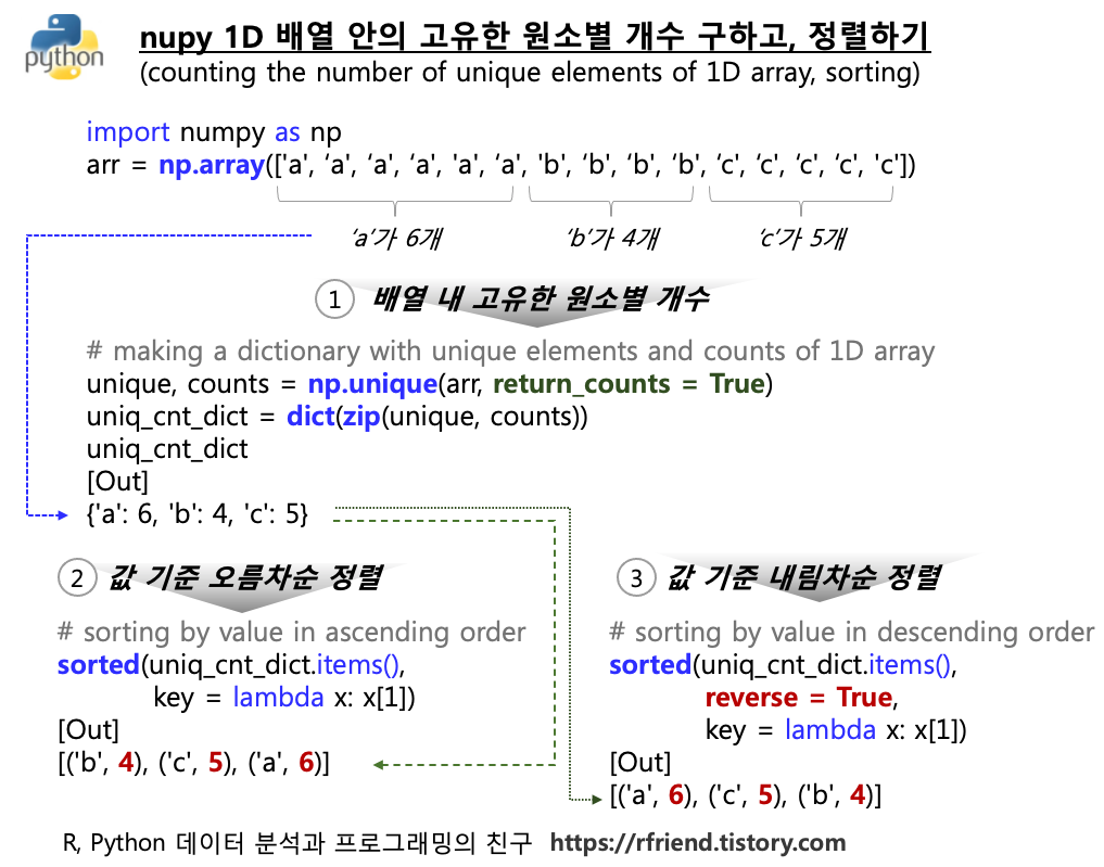
먼저 np.unique(arr, return_counts = True) 의 결과를 unique, counts 라는 이름의 array로 할당을 받고, 이를 zip(unique, counts) 으로 쌍(pair)을 만들어준 다음에, dict() 를 사용해서 사전형으로 변환해주었습니다.
## making a dictionary with unique elements and counts of 1D array
unique, counts = np.unique(arr, return_counts = True)
uniq_cnt_dict = dict(zip(unique, counts))

uniq_cnt_dict
[Out]
{'a': 6, 'b': 4, 'c': 5}
(4) numpy 1D 배열의 고유한 원소(key) 별 개수(value)의 사전을 정렬하기
(sorting a dictionary with unique sets and counts of 1D numpy array)
위의 (3)번까지 잘 진행을 하셨다면 이제 (unique : counts) 쌍의 사전을 'counts' 의 값을 기준으로 오름차순 정렬(sorting a dict by value in ascending order) 또는 내림차순 정렬 (sorting a dict by value in descending order) 하고 싶은 마음이 생길 수 있는데요, 이럴 경우 sorted() 메소드를 사용하면 되겠습니다. (pytho dictionary 정렬 참조: rfriend.tistory.com/473)
## sorting a dictionary by value in ascending order
## -- reference: https://rfriend.tistory.com/473
sorted(uniq_cnt_dict.items(),
       key = lambda x: x[1])

[Out]
[('b', 4), ('c', 5), ('a', 6)]


## sorting a dictionary by value in descending order
sorted(uniq_cnt_dict.items(),
       reverse = True,
       key = lambda x: x[1])

[Out]
[('a', 6), ('c', 5), ('b', 4)]
(5) numpy 1D 배열을 pandas Series 로 변환해 고유한 원소별 개수 구하고 정렬하기
(converting 1D array to pandas Series, and value_counts(), sort_values())
pandas 의 Series 나 DataFrame으로 변환해서 데이터 분석 하는 것이 더 익숙하거나 편리한 상황에서는 pandas.Series(array) 나 pandas.DataFrame(array) 로 변환을 해서, value_count() 메소드로 원소의 개수를 세거나, sort_values() 메소드로 값을 기준으로 정렬을 할 수 있습니다.
import pandas as pd

## converting an array to pandas Series
arr_s = pd.Series(arr)
arr_s
[Out]
0     a
1     c
2     c
3     b
4     a
5     b
6     b
7     c
8     a
9     c
10    b
11    a
12    a
13    a
14    c
dtype: object


## counting values by unique elements of pandas Series
arr_s.value_counts()
[Out]
a    6
c    5
b    4
dtype: int64


## sorting by values in ascending order of pandas Series
arr_s.value_counts().sort_values(ascending=True)
[Out]
b    4
c    5
a    6
dtype: int64
(converting 1D array to pandas DataFrame, and value_counts(), sort_values())
만약 pandas Series 내 고유한 원소별 개수를 구한 결과를 개수의 오름차순으로 정렬을 하고 싶다면 sort_values(ascending = True) 를 설정해주면 됩니다. (내림차순이 기본 설정, default to descending order)
import pandas as pd

## converting an array to pandas DataFrame
arr_df = pd.DataFrame(arr, columns=['x1'])
arr_df

[Out]
x1
0	a
1	c
2	c
3	b
4	a
5	b
6	b
7	c
8	a
9	c
10	b
11	a
12	a
13	a
14	c


## counting the number of unique elements in Series
arr_df['x1'].value_counts()
[Out]
a    6
c    5
b    4
Name: x1, dtype: int64


## # sorting by the counts of unique elements in ascending order
arr_df['x1'].value_counts().sort_values(ascending=True)
[Out]
b    4
c    5
a    6
Name: x1, dtype: int64
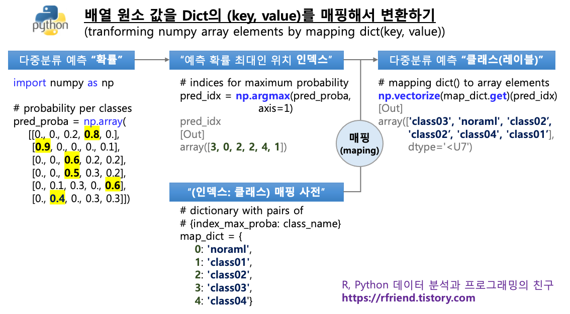
이들 확률값 배열로 부터 하나의 예측값을 구하기 위해 이들 5개 각 class별 확률 중에서 가장 큰 값을 가지는 위치 (indices of maximum value) 의 class 를 모델이 예측한 class 라고 정의해보겠습니다.
np.argmax(pred_proba, axis=1) 은 배열 내의 각 관측치 별 (axis = 1) 로 가장 큰 확률값의 위치의 인덱스를 반환합니다. 가령, 위의 pred_proba 의 첫번째 관측치의 5개 class 별 속할 확률은 [0., 0., 0.2, 0.8, 0.] 의 배열로서, 확률 0.8 이 가장 큰 값이므로 위치 인덱스 '3'을 반환하였습니다.
## positional index for maximum probability
pred_idx = np.argmax(pred_proba, axis=1)
pred_idx
[Out]
array([3, 0, 2, 2, 4, 1])
(2) np.vectorize() 와 dict.get() 을 사용해서 최대값 위치 인덱스와 분류 레이블을 매핑하기
위의 (1)번에서 구한 확률 최대값의 위치 인덱스 가지고, 이번에는 아래의 'class_map_dict'와 같이 {키: 값} 쌍 사전의 '키(key)'를 기준으로 매핑을 해서, 다중분류 모델의 예측값을 'class 이름'으로 변환을 해보겠습니다.
이때 dict.get(key) 를 유용하게 사용할 수 있습니다. dict.get(key) 메소드는 사전(dict)의 키에 쌍으로 대응하는 값을 반환해줍니다. 따라서 바로 위에서 정의해준 'class_map_dict'의 키 값을 넣어주면, 각 키에 해당하는 'normal'~'class04' 의 사전 값을 반환해줍니다.
## get() returns the value for the specified key if key is in dict.
class_map_dict.get(pred_idx[0])
[Out]
'class03'


class_map_dict.get(0)
[Out]
'noraml'
사전의 (키: 값)을 매핑하려는 배열 내 원소가 많을 경우, np.vectorize() 메소드를 이용하면 매우 편리하고 또 빠르게 사전의 (키: 값)을 매핑을 해서 배열의 값을 변환할 수 있습니다. 아래 예에서는 'class_map_dict' 의 (키: 값) 사전을 사용해서 'pred_idx'의 확률 최대값 위치 인덱스 배열을 'pred_cls' 의 예측한 클래스(레이블) 이름('normal'~'class04')으로 변환해주었습니다.
np.vectorize() 는 numpy의 broadcasting 규칙을 사용해서 매핑을 하므로 코드가 깔끔하고, for loop을 사용하지 않으므로 원소가 많은 배열을 처리해야 할 경우 빠릅니다.
## vectorization of dict.get(array_idx) for all elements of array
pred_cls = np.vectorize(class_map_dict.get)(pred_idx)

pred_cls
[Out]
array(['class03', 'noraml', 'class02', 'class02', 'class04', 'class01'],
      dtype='<U7')
(3) for loop 과 dict.get() 을 사용해서 최대값 위치 인덱스와 분류 레이블을 매핑하기
만약 위의 (2)번 처럼 np.vectorize() 메소드를 사용하지 않는다면, 아래처럼 for loop 사용해서 확률 최대값 위치 인덱스의 개수 만큼 순환 반복을 하면서 dict.get() 함수를 적용해주어야 합니다. 위의 (2)번 대비 코드도 길고, 또 대상 배열이 클 경우 시간도 더 오래 걸리므로 np.vectorize() 사용을 권합니다.
## manually using for loop
pred_cls_mat = np.empty(pred_idx.shape, dtype='object')

for i in range(len(pred_idx)):
    pred_cls_mat[i] = class_map_dict.get(pred_idx[i])

pred_cls_mat
[Out]
array(['class03', 'noraml', 'class02', 'class02', 'class04', 'class01'],
      dtype=object)