이번 포스팅에서는 Python의 SciPy 모듈을 사용해서 각 원소 간 짝을 이루어서 유클리디언 거리를 계산(calculating pair-wise distances)하는 방법을 소개하겠습니다. 본문에서 scipy 의 거리 계산함수로서 pdist()와 cdist()를 소개할건데요, 반환하는 결과물의 형태에 따라 적절한 것을 선택해서 사용하면 되겠습니다. 마지막으로 scipy 에서 제공하는 거리를 계산하는 기준(distance metric)에 대해서 알아보겠습니다. 

(Scikit-Learn 모듈에도 거리 계산 함수가 있는데요, SciPy 모듈에 거리 측정 기준이 더 많아서 SciPy 모듈로 소개합니다.) 


(1) scipy.spatial.distance.pdist(): returns condensed distance matrix Y.

(2) scipy.spatial.distance.cdist(): returns M by N distance matrix.

(3) 거리 측정 기준(distance metric)


calculating pair-wise distances using python SciPy


먼저, 예제로 사용할 간단한 샘플 데이터셋으로서 x와 y의 두 개의 칼럼에 대해 4개의 원소를 가지는 numpy array 로 만들어보겠습니다. 그리고 matplotlib 으로 산점도를 그려서 4개의 원소에 대해 x와 y의 좌표에 산점도를 그려서 확인해보겠습니다. 


ID x y
1 3 2
2 3 3
3 5 5
4 6 7


import numpy as np
import matplotlib.pyplot as plt

X = np.array([
    # x, y
    [3, 2], # ID 1
    [3, 3], # ID 2
    [5, 5], # ID 3
    [6, 7], # ID 4
])

plt.plot(X[:, 0], X[:, 1], 'o')
plt.show()

scatter plot


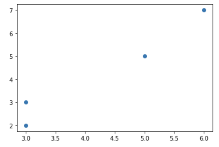
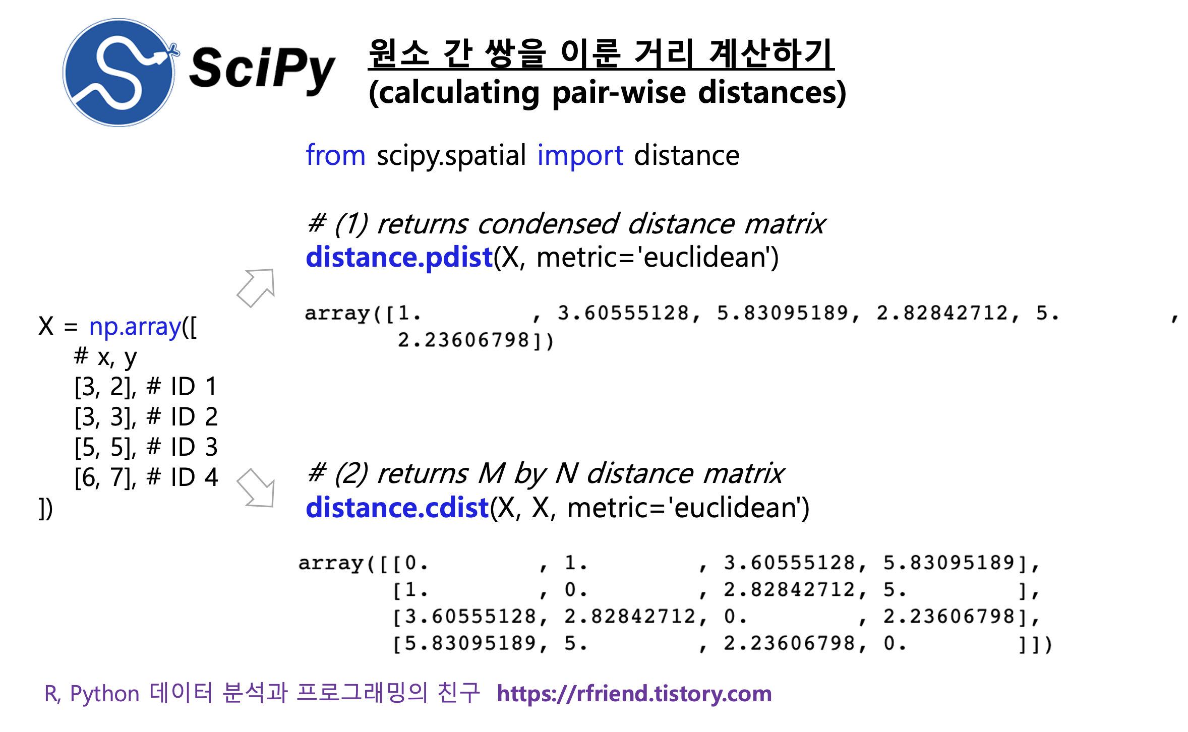
(1) scipy.spatial.distance.pdist(X, metric='euclidean'): returns condensed distance matrix Y.


scipy.spatial.distance.pdist(X, metric='euclidean') 함수는 X 벡터 또는 행렬에서 각 원소(관측치) 간 짝을 이루어서 유클리디언 거리를 계산해줍니다. 그리고 응축된 형태의 거리 행렬(condensed distance matrix)을 반환합니다. 아래의 (1)번 pdist() 계산 결과가 반환된 형태를 (2) cdist() 로 계산 결과가 반환된 형태와 비교해보면 이해가 쉬울 거예요. 


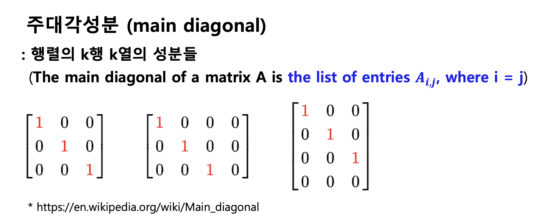
pdist(X, metric='eudlidean') 계산 결과는 각 관측치 간 짝을 이룬 거리 계산이므로 아래 값들의 계산 결과입니다. 거리 계산 결과는 자기 자신과의 거리인 대각행렬 부분은 제외하고, 각 원소 간 쌍을 이룬 부분에 대해서만 관측치의 순서에 따라서 반환되었습니다. (예: ID1 : ID2, ID1 : ID3, ID1 : ID4, ID2 : ID3, ID2 : ID4, ID3 : ID4)


   * DISTANCE_euclidean(ID 1, ID 2) = sqrt((3-3)^2 + (2-3)^2) = 1.00

   * DISTANCE_euclidean(ID 1, ID 3) = sqrt((3-5)^2 + (2-5)^2) = 3.60

   * DISTANCE_euclidean(ID 1, ID 4) = sqrt((3-6)^2 - (2-7)^2) = 5.83

   * DISTANCE_euclidean(ID 2, ID 3) = sqrt((3-5)^2 - (3-5)^2) = 2.82

   * DISTANCE_euclidean(ID 2, ID 4) = sqrt((3-6)^2 - (3-7)^2) = 5.00

   * DISTANCE_euclidean(ID 3, ID 4) = sqrt((5-6)^2 - (5-7)^2) = 2.23


# scipy.spatial.distance.pdist(X, metric='euclidean', *, out=None, **kwargs)
# : Pairwise distances between observations in n-dimensional space.
# : Returns a condensed distance matrix Y.

from scipy.spatial import distance

X_pdist = distance.pdist(X, metric='euclidean')

X_pdist
# array([1.        , 3.60555128, 5.83095189, 2.82842712, 5.        ,
#        2.23606798])


(2) scipy.spatial.distance.cdist(): returns M by N distance matrix.


scipy.spatial.distance.cdist(XA, XB, metric='euclidean') 함수는 원소(관측치) 간 쌍을 이루어 유클리디언 거리를 계산합니다만, 위의 (1) pdist() 함수와는 달리, 


  - (a) input 으로 XA, XB 의 두 개의 행렬 (혹은 벡터)를 받으며, (vs. pdist() 는 X 행렬 한 개만 받음)

  - (b) output 으로 M by N 거리 행렬을 반환합니다. (vs. pdist() 는 condensed distance matrix 를 반환)


하는 차이점이 있습니다.  위의 (1)번 scipy.spatial.distance.pdist() 함수와 (2) scipy.spatial.distance.cdist() 함수의 input, output을 비교해보면 이해가 쉬울 거예요. 


# scipy.spatial.distance.cdist(XA, XB, metric='euclidean', *, out=None, **kwargs)
# : Compute distance between each pair of the two collections of inputs.
# : A M by N distance matrix is returned.(M for X, N for Y)

from scipy.spatial import distance

X_cdist = distance.cdist(X, X, metric='euclidean')
X_cdist
# array([[0.        , 1.        , 5.83095189, 3.60555128],
#        [1.        , 0.        , 5.        , 2.82842712],
#        [5.83095189, 5.        , 0.        , 2.23606798],
#        [3.60555128, 2.82842712, 2.23606798, 0.        ]])


(3) 거리 측정 기준(distance metric)


위의 (1), (2)번에서는 거리 측정 기준으로 디폴트 옵션인 '유클리디언 거리(metric='euclidean distance') 를 사용해서 원소 간 쌍을 이룬 거리를 계산하였습니다. 


scipy 모듈은 유클리디어 거리 외에도 다양한 거리 측정 기준을 제공합니다. (맨하탄 거리, 표준화 거리, 마할라노비스 거리, 자카드 거리, 코사인 거리, 편집 거리에 대해서는 아래의 Reference 의 링크를 참고하세요.)


[ scipy.spatial.distance.pdist(), cdist() 함수의 metric options (알파벳 순서) ]

‘braycurtis’, ‘canberra’, ‘chebyshev’, ‘cityblock’, ‘correlation’, ‘cosine’, ‘dice’, ‘euclidean’, ‘hamming’, ‘jaccard’, ‘jensenshannon’, ‘kulsinski’, ‘kulczynski1’, ‘mahalanobis’, ‘matching’, ‘minkowski’, ‘rogerstanimoto’, ‘russellrao’, ‘seuclidean’, ‘sokalmichener’, ‘sokalsneath’, ‘sqeuclidean’, ‘yule’.


아래에는 metric='cityblcok' 매개변수 설정을 통해서 '맨하탄 거리(Manhattan distance)'를 계산하여 보았습니다. cdist() 함수를 사용하였으므로 4 by 4 행렬의 형태로 관측치 간 쌍을 이룬 거리 계산 결과를 반환합니다. 


   * DISTANCE_manhattan(ID 1, ID 2) = |3-3|+|2-3| = 1

   * DISTANCE_manhattan(ID 1, ID 3) = |3-5|+|2-5| = 5

   * DISTANCE_manhattan(ID 1, ID 4) = |3-6|+|2-7| = 8

   * DISTANCE_manhattan(ID 2, ID 3) = |3-5|+|3-5| = 4

   * DISTANCE_manhattan(ID 2, ID 4) = |3-6|+|3-7| = 7

   * DISTANCE_manhattan(ID 3, ID 4) = |5-6|+|5-7| = 3


X
# array([[3, 2],
#        [3, 3],
#        [5, 5],
#        [6, 7]])


## Manhattan Distance
from scipy.spatial import distance

X_cdist_cityblock = distance.cdist(X, X, metric='cityblock')

X_cdist_cityblock
# array([[0., 1., 5., 8.],
#        [1., 0., 4., 7.],
#        [5., 4., 0., 3.],
#        [8., 7., 3., 0.]])


[ Reference ]


[1] scipy.spatial.distance.pdist
https://docs.scipy.org/doc/scipy/reference/generated/scipy.spatial.distance.pdist.html#scipy.spatial.distance.pdist
[2] scipy.spatial.distance.cdist
https://docs.scipy.org/doc/scipy/reference/generated/scipy.spatial.distance.cdist.html#scipy.spatial.distance.cdist
[3] 맨하탄 거리(Manhattan distance), 유클리드 거리(Euclidean distance), 표준화 거리(), 마할라노비스 거리
https://rfriend.tistory.com/199
[4] 자카드 거리 (Jaccard distance): https://rfriend.tistory.com/318
[5] 코사인 거리 (cosine distance): https://rfriend.tistory.com/319
[6] 편집거리 (edit distance, Levenshtein metric): https://rfriend.tistory.com/320


이번 포스팅이 많은 도움이 되었기를 바랍니다. 

행복한 데이터 과학자 되세요!  :-)


728x90
반응형
Posted by Rfriend
,

주대각성분 또는 주대각선 (main diagonal, leading diagonal, principal diagonal, primary diagonal, major diagonal) 은 행렬의 k행 k열의 성분들을 말합니다. 


대각행렬(diagonal matrix) 및 그외 특수한 행렬에 대해서는 https://rfriend.tistory.com/141 를 참고하세요. 


 mail diagonal


이번 포스팅에서는 Python NumPy 를 이용해서 주대각성분(main diagonal)을 다루는 방법을 소개하겠습니다. 


(1) 주대각성분 가져오기 (returning a main diagonal)

(2) 주대각성분을 기준으로 수평/ 수직으로 뒤집기 (flip horizontally/ vertically by main diagonal) 

(3) 주대각성분 채우기 (filling main diagonal) 

(4) 대각행렬 만들기 (creating a diagonal matrix) 


(1) 주대각성분 가져오기 (returning a main diagonal): np.diagonal()


import numpy as np

## making a sample 2-D array
arr = np.arange(9).reshape(3, 3)
arr
# array([[0, 1, 2],
#        [3, 4, 5],
#        [6, 7, 8]])


## (1) main diagonal
np.diagonal(arr)
# array([0, 4, 8])


## (2) main diagonal
arr.diagonal()
# array([0, 4, 8])


(2) 수평/ 수직으로 뒤집은 후 주대각성분 가져오기 (returning main diagonal after flipping) 


(2-1) 수평으로 뒤집은 후 주대각성분 가져오기 (returning main diagonal after flipping horizontally)
          : np.fliplr(arr).diagonal()


# Horizontal flip
np.fliplr(arr) # flip from left to right
# array([[2, 1, 0],
#        [5, 4, 3],
#        [8, 7, 6]])


## main diagonal of horizontal flip
np.fliplr(arr).diagonal()
# array([2, 4, 6])


(2-2) 수직으로 뒤집은 후 주대각성분 가져오기 (returning main diagonal after flipping vertically)
         : np.flipud(arr).diagonal()


# Vertical flip
np.flipud(arr) # flip from up to down
# array([[6, 7, 8],
#        [3, 4, 5],
#        [0, 1, 2]])


## main diagonal of vertical flip
np.flipud(arr).diagonal()
# array([6, 4, 2])


(3) 주대각성분 채우기 (filling main diagonal)  : np.fill_diagonal()


## filling the main diagonal of the given array of any dimensionality
## using np.fill_diagonal(a, val)
np.fill_diagonal(arr, val=999)


arr
# array([[999,   1,   2],
#        [  3, 999,   5],
#        [  6,   7, 999]])


(4) 대각행렬 만들기 (creating a diagonal matrix)  


대각행렬(diagonal matrix)은 주대각성분에만 원소 값이 있고, 주대각성분 외의 원소는 값이 모두 '0'인 행렬을 말합니다.

아래의 예에서는 NumPy로 대각행렬을 만들기 위해서, 먼저 np.zeros([m, n]) 로 '0'의 값만을 가지는 m by n 행렬을 만든 후에, np.fill_diagonal(array, val) 의 val 부분에 원하는 주대각성분의 값(예: val=[1, 2, 3])을 입력해주어서 대각행렬(diag(1, 2, 3))을 만들어 보겠습니다. 


## making a diagonal matrix: diag(1, 2, 3)
arr2 = np.zeros([3, 3])
arr2
# array([[0., 0., 0.],
#        [0., 0., 0.],
#        [0., 0., 0.]])


## filling main diagonal with [1, 2 3] values using np.fill_diagonal()
np.fill_diagonal(arr2, val=[1, 2, 3])

arr2
# array([[1., 0., 0.],
#        [0., 2., 0.],
#        [0., 0., 3.]])


[ Reference ]

1. 주대각성분 (또는 주대각선, main diagonal)
    : https://en.wikipedia.org/wiki/Main_diagonal 

2. numpy.diagonal()
    : https://numpy.org/doc/stable/reference/generated/numpy.diagonal.html

3. numpy.fill_diagonal()
    : https://numpy.org/doc/stable/reference/generated/numpy.fill_diagonal.html

4. 대각행렬(diagonal matrix) 및 특수행렬: https://rfriend.tistory.com/141


이번 포스팅이 많은 도움이 되었기를 바랍니다. 

행복한 데이터 과학자 되세요!  :-)


728x90
반응형
Posted by Rfriend
,

이번 포스팅에서는 Python pandas의 문자열 Series에서 문자열 패턴 매칭을 통해서 특정 패턴이 포함되어 있는지 여부를 확인하고, 특정 매칭을 포함한 데이터를 가져오는 방법을 소개하겠습니다. 


(1) pandas 문자열 Series에서 한개의 문자열 패턴 매칭하기 
     : Series.str.contains(pattern)

(2) pandas DataFrame에서 한개의 문자열 패턴 매칭이 되는 데이터 가져오기

(3) pandas DataFrame에서 여러개의 문자열 패턴 매팅이 되는 데이터 가져오기


먼저, 예제로 사용할 문자열이 포함된 DataFrame을 만들어보겠습니다. pandas 의 contains() 함수를 사용해서 문자열 뿐만 아니라 NaN 값과 '1004' 숫자도 포함시켜서 문자열 매칭 시 처리방법을 소개하겠습니다. 


## importing modules
import numpy as np
import pandas as pd

## creating a pandas DataFrame with strings, NaN, digit
df = pd.DataFrame({
    'id': [1, 2, 3, 4, 5, 6, 7]
    , 'fruit': ['apple', 'PERSIMON', 'grapes', 'mango', 'peach and perl', 
                np.NaN, 
                '1004']
})


print(df)
#    id           fruit
# 0   1           apple
# 1   2        PERSIMON
# 2   3          grapes
# 3   4           mango
# 4   5  peach and perl
# 5   6             NaN
# 6   7            1004


(1) pandas 문자열 Series에서 한개의 문자열 패턴 매칭하기: Series.str.contains(pattern)


먼저, 위에서 만든 DataFrame에서 'fruit' 칼럼만 가져와서 's1' 이라는 이름의 Series 를 만들어보겠습니다. 


## pandas Series
s1 = df['fruit']

print(type(s1)) # padnas.Series
print(s1)

# <class 'pandas.core.series.Series'>
# 0             apple
# 1          PERSIMON
# 2            grapes
# 3             mango
# 4    peach and perl
# 5               NaN
# 6              1004
# Name: fruit, dtype: object


pandas 의 contains() 메소드는 '문자열 Series (Series of a string)' 을 대상으로 문자열 매칭을 해서 Boolean Series 를 반환합니다. contains() 메소드의 구문은 아래와 같습니다. 


Series.str.contains(pattern, case=True, flags=0, na=None, regex=True)


이때 Series.str.contains() 메소드는 문자열 Series에 대하여 패턴 매칭(pattern matching)을 할 때 문자열 그 자체(literal itself)와 함께 정규표현식(regex=True: regular expression)까지도 사용해서 패턴 매칭을 할 수 있으며, '대/소문자 구분 (case=True: case sensitive)하며, 'NaN' 값에 대해서는 'NaN'을 반환(na=None)합니다. 


아래 예에서는 문자열 Series 's1'에 대해서 문자열 'pe'가 들어있는 패턴 매칭을 해서 Boolean Series 를 반환한 예입니다. (대소문자 구분, NaN은  NaN 반환) 


## returning a Series of Booleans using a literal pattern
s1.str.contains('pe')

# 0    False
# 1    False   # <-- case sensitive
# 2     True
# 3    False
# 4     True
# 5      NaN   # <-- returning NaN for NaN values
# 6    False
# Name: fruit, dtype: object


(2) pandas DataFrame에서 한개의 문자열 패턴 매칭이 되는 데이터 가져오기


pandas DataFrame에서 특정 문자열 칼럼에 대해서 문자열 패턴 매칭한 결과인 Boolean Series 를 이용해서 해당 행의 값만 가져올 수 있습니다. 이때 만약 문자열 패턴 매칭 결과 Boolean Seires 에 NaN 값이 포함되어 있을 경우 아래와 같은 ValueError 가 발생합니다. 


ValueError: Cannot mask with non-boolean array containing NA / NaN valu


 ## ValueError: Cannot mask with non-boolean array containing NA / NaN values
df[df['fruit'].str.contains('pe')]

---------------------------------------------------------------------------
ValueError                                Traceback (most recent call last)
<ipython-input-5-ee5e3bc73f2f> in <module>
      1 ## ValueError: Cannot mask with non-boolean array containing NA / NaN values
----> 2 df[s1.str.contains('pe')]

~/opt/anaconda3/lib/python3.8/site-packages/pandas/core/frame.py in __getitem__(self, key)
   2890 
   2891         # Do we have a (boolean) 1d indexer?
-> 2892         if com.is_bool_indexer(key):
   2893             return self._getitem_bool_array(key)
   2894 

~/opt/anaconda3/lib/python3.8/site-packages/pandas/core/common.py in is_bool_indexer(key)
    132                 na_msg = "Cannot mask with non-boolean array containing NA / NaN values"
    133                 if isna(key).any():
--> 134                     raise ValueError(na_msg)
    135                 return False
    136             return True

ValueError: Cannot mask with non-boolean array containing NA / NaN values


'ValueError: Cannot mask with non-boolean array containing NA/NaN values' 를 해결하기 위해서는 Series.str.contains(pattern, na=False) 처럼 NaN 값을 Boolean의 'False'로 설정해주면 됩니다. 


## Specifying na to be False instead of NaN replaces NaN values with False.
df[df['fruit'].str.contains('pe'
                   , na=False) # specifying NA to be False
  ]

#  id	fruit
# 2	3	grapes
# 4	5	peach and perl


만약 문자열 매칭을 할 때 '대/소문자 구분없이 (case insensitive)' 하려면 'case=False' 옵션을 설정해주면 됩니다. 

아래 예에서는 case=False 로 설정한 상태에서 'pe' 문자열 매칭을 했더니 'PERSIMON' 대문자도 매칭이 되어서 가져오기가 되었습니다. 


## Specifying case sensitivity using case.
df[df['fruit'].str.contains('pe'
                   , na=False
                   , case=False) # case = False
  ] 

#   id	fruit
# 1	2	PERSIMON   # <-- case insensitive
# 2	3	grapes
# 4	5	peach and perl


Series.str.contains() 함수에는 정규표현식(regex=True: Regular Expression)을 사용해서 문자열 매칭을 할 수 있습니다.  아래의 예에서는 정규표현식을 이용해서 '숫자가 포함된 ('\\d' : returning any digits)' 문자열을 가져와보겠습니다. 


## returning any digit using regular expression
df[df['fruit'].str.contains(
    '\\d'        # returning any digit
    , regex=True # using regular expression
    , na=False
    )
  ]

#   id	fruit
# 6	7	1004


(3) pandas DataFrame에서 여러개의 문자열 패턴 매팅이 되는 데이터 가져오기


이번에는 문자열 매칭을 할 때 '여러개의 문자열 패턴 (multiple strings of pattern)' 과 매칭되는 문자열을 확인하고, pandas DataFrame으로 부터 해당 행의 데이터를 가져와보겠습니다. 


여러개의 문자열 패턴을 표현할 때 '|' 가 'or' 를 나타냅니다. 아래의 예의 경우, ['ap' or 'ma' or 'gr'] 이 포함된 문자열을 매칭해서 Boolean String을 반환하고 싶을 때 ['ap'|'ma'|'gr'] 을 패턴으로 입력해주면 됩니다. Python의 내장함수(built-in function) 중에서 join() 메소드를 이용하면 여러개의 문자열을 '|' 구분자(separator)를 넣어서 하나의 문자열로 묶어줄 수 있습니다. ('|'.join(['ap', 'ma', 'gr']) 은 ==> 'ap|ma|gr' 을 반환하며, ==> ['ap' or 'ma' or 'gr'] 을 의미함)


## join() method joins all itmes in a tuple into a string with a separartor
'|'.join(['ap', 'ma', 'gr'])

# 'ap|ma|gr'


## Returning ‘apple’ or ‘mango’ or 'grapes' 
## when either expression occurs in a string.
s1.str.contains(
    '|'.join(['ap', 'ma', 'gr']) # 'ap|ma|gr', ie. 'ap' or 'ma' or 'gr'
    , na=False
    , case=False
)

# 0     True
# 1    False
# 2     True
# 3     True
# 4    False
# 5    False
# 6    False
# Name: fruit, dtype: bool


이제 pandas DataFrame 에서 'fruit' 칼럼에서 'ap' or 'ma' or 'gr' 문자열이 포함되어 있는 모든 행을 가져와보겠습니다. 


## indexing data using a Series of Booleans 
df[df['fruit'].str.contains(
    '|'.join(['ap', 'ma', 'gr'])
    , na=False
    , case=False
    )
  ]

#   id	fruit
# 0	1	apple
# 2	3	grapes
# 3	4	mango


[ Reference ]

[1] pandas.Series.str.contains()
    : https://pandas.pydata.org/docs/reference/api/pandas.Series.str.contains.html


이번 포스팅이 많은 도움이 되었기를 바랍니다. 

행복한 데이터 과학자 되세요!  :-)


728x90
반응형
Posted by Rfriend
,

탐색적 데이터 분석 및 데이터 전처리를 할 때 특정 행과 열을 기준으로 데이터를 선택(selection), 인덱싱(indexing), 슬라이싱(slicing)하는 하는 처리가 필요합니다. 이때 pandas 에서 사용할 수 있는 게 loc, iloc 인데요, 비슷해서 좀 헷갈리는 면이 있습니다. 


이번 포스팅에서는 Python pandas 의 DataFrame에서 데이터를 선택(selection), 인덱싱(indexing), 슬라이싱(slicing)할 때 사용하는 loc vs. iloc 를 비교해보겠습니다. 


- loc 는 레이블 기반 (label-based) 또는 블리언 배열(boolean array) 기반으로 데이터를 선택 

- iloc 는 정수 기반의 위치 (integer-based position) 또는 블리언 배열(boolean array) 기반으로 데이터를 선택


아래의 순서대로 loc vs. iloc 를 간단한 예를 들어 비교하면서 소개하겠습니다. 

(1) A Value

(2) A List or Array

(3) A Slice Object

(4) Conditions or Boolean Array

(5) A Callable Function


[ Pandas DataFrame의 데이터를 선택할 때 사용하는 loc vs. iloc ]

selecting data in pandas DataFrame using loc vs. iloc


먼저, index를 수기 입력해주고, 숫자형과 범주형 변수를 모두 가지는 간단한 예제 pandas DataFrame을 만들어보겠습니다. 


## creating a sample pandas DataFrame
import pandas as pd

df = pd.DataFrame({
    'name': ['park', 'choi', 'lee', 'kim', 'lim', 'yang'], 
    'gender': ['M', 'F', 'F', 'M', 'F', 'F'], 
    'age': [25, 29, 25, 31, 38, 30], 
    'grade': ['S', 'B', 'C', 'A', 'D', 'S'], 
    'tot_amt': [500, 210, 110, 430, 60, 680]}, 
    index=['c100', 'c101', 'c102', 'c103', 'c104', 'c105'])


print(df)
#       name gender  age grade  tot_amt
# c100  park      M   25     S      500
# c101  choi      F   29     B      210
# c102   lee      F   25     C      110
# c103   kim      M   31     A      430
# c104   lim      F   38     D       60
# c105  yang      F   30     S      680


아래부터는 loc vs. iloc 코드 예시인데요, 모두 데이터를 선택하는 굉장히 간단한 코드들 이므로 설명은 생략합니다. 특이사항에 대해서만 간략히 부연설명 남겨요. 


(1) loc vs. iloc: A Value


한 개의 행 레이블(a single row label)로 loc 를 사용해서 값을 가져오면 pandas Series 를 반환하는 반면에, 리스트(list, [ ]) 안에 1개 행 레이블을 넣어서 loc 를 사용하면 pandas DataFrame을 반환합니다. 이것은 iloc 에 정수 위치를 넣어서 값을 가져올 때도 동일합니다. 


## (1) pandas.DataFrame.loc[]
## : Access a group of rows and colmns by label(s) or a boolean array

## (1-1) using a row label --> returns a pandas Series
df.loc['c100']
# name       park
# gender        M
# age          25
# grade         S
# tot_amt     500
# Name: c100, dtype: object


## (1-2) using a list of row label --> returns a pandas DataFrame
df.loc[['c100']]
#       name gender  age grade  tot_amt
# c100  park      M   25     S      500


## (2) pandas.DataFrame.iloc[]
## : Purely integer-location based indexing for selection by position.

## (2-1) A scalar of integer --> returns pandas Series
df.iloc[0]
# name       park
# gender        M
# age          25
# grade         S
# tot_amt     500
# Name: c100, dtype: object


## (2-2) A list of integer --> returns pandas DataFrame
df.iloc[[0]]
#       name gender  age grade  tot_amt
# c100  park      M   25     S      500


(2) loc vs. iloc: A List or Array


df.loc[['c100', 'c105']] 처럼 loc 에 레이블 리스트를 사용하면 해당 행의 다수의 열의 값을 가져오며, df.loc['c100', 'name'] 처럼 사용하면 레이블 기반의 해당 행(row)과 열(column)의 값을 가져옵니다. 


## (1) pandas.DataFrame.loc[]
## : Access a group of rows and colmns by label(s) or a boolean array

## (1-2) using multiple row labels
df.loc[['c100', 'c105']]
#       name gender  age grade  tot_amt
# c100  park      M   25     S      500
# c105  yang      F   30     S      680


## using row and column label
df.loc['c100', 'name']
# 'park'


## (2) pandas.DataFrame.iloc[]
## : Purely integer-location based indexing for selection by position.

## (2-2) A list or array of integers
df.iloc[[0, 1, 3, 5]]
#       name gender  age grade  tot_amt
# c100  park      M   25     S      500
# c101  choi      F   29     B      210
# c103   kim      M   31     A      430
# c105  yang      F   30     S      680


(3) loc vs. iloc: A Slice Object


loc 로 레이블 기반 슬라이싱을 하면 처음과 끝 레이블 값이 포함된 채로 값을 가져옵니다. 예를 들어, 아래의 df.loc['c100':'c103'] 은 'c100'과 'c103' 행도 모두 포함된 값을 가져왔습니다. 반면에 iloc 로 정수 위치 기반으로 슬라이싱을 하면 처음 정수 위치의 행은 가져오지만 마지막의 정수 위치의 행은 가져오지 않습니다. 


## (1) pandas.DataFrame.loc[]
## : Access a group of rows and colmns by label(s) or a boolean array

## (1-3) Slice with labels for row and single label for column.
df.loc['c100':'c103', 'name']
# c100    park
# c101    choi
# c102     lee
# c103     kim
# Name: name, dtype: object


## (2) pandas.DataFrame.iloc[]
## : Purely integer-location based indexing for selection by position.

## (2-3) slicing using integer
df.iloc[1:4]
#       name gender  age grade  tot_amt
# c101  choi      F   29     B      210
# c102   lee      F   25     C      110
# c103   kim      M   31     A      430


(4) loc vs. iloc: Conditions or Boolean Array


loc 의 레이블 기반 데이터 선택에는 조건문과 블리언 배열을 모두 사용할 수 있습니다. iloc 의 정수 기반 데이터 선택에는 블리언 배열을 사용할 수 있습니다. 


## (1) pandas.DataFrame.loc[]
## : Access a group of rows and colmns by label(s) or a boolean array

## (1-4-1) Conditional that returns a boolean Series

## Boolean list with the same length as the row axis
df['tot_amt'] > 400
# c100     True
# c101    False
# c102    False
# c103     True
# c104    False
# c105     True
# Name: tot_amt, dtype: bool


## Conditional that returns a boolean Series
df.loc[df['tot_amt'] > 400]
#       name gender  age grade  tot_amt
# c100  park      M   25     S      500
# c103   kim      M   31     A      430
# c105  yang      F   30     S      680


## Conditional that returns a boolean Series with column labels specified
df.loc[df['tot_amt'] > 400, ['name']]
#       name
# c100  park
# c103   kim
# c105  yang


## (1-4-2) A boolean array
df.loc[[True, False, False, True, False, True]]
#       name gender  age grade  tot_amt
# c100  park      M   25     S      500
# c103   kim      M   31     A      430
# c105  yang      F   30     S      680


## (2) pandas.DataFrame.iloc[]
## : Purely integer-location based indexing for selection by position.

## (2-4) With a boolean mask the same length as the index. 
## loc and iloc are interchangeable when labels are 0-based integers.
df.iloc[[True, False, False, True, False, True]]
#       name gender  age grade  tot_amt
# c100  park      M   25     S      500
# c103   kim      M   31     A      430
# c105  yang      F   30     S      680


(5) loc vs. iloc: A Callable Function


lambda 익명함수를 사용하여 호출 가능한 함수를 loc, iloc 에 사용해서 값을 선택할 수 있습니다. 

(df.iloc[lambda df: df['tot_amt'] > 400] 은 왜그런지 모르겠는데 에러가 나네요. -_-;)


## (1) pandas.DataFrame.loc[]
## : Access a group of rows and colmns by label(s) or a boolean array

## (1-5) Callable that returns a boolean Series
df.loc[lambda df: df['tot_amt'] > 400]
#       name gender  age grade  tot_amt
# c100  park      M   25     S      500
# c103   kim      M   31     A      430
# c105  yang      F   30     S      680


## (2) pandas.DataFrame.iloc[]
## : Purely integer-location based indexing for selection by position.

## (2-7) Callable that returns a boolean Series
df.iloc[lambda x: x.index == 'c100']
#       name gender  age grade  tot_amt
# c100  park      M   25     S      500


[ Reference ]

* pandas DataFrame에서 행, 열 데이터 선택: https://rfriend.tistory.com/282 
* pandas loc: https://pandas.pydata.org/docs/reference/api/pandas.DataFrame.loc.html   
* pandas iloc: https://pandas.pydata.org/docs/reference/api/pandas.DataFrame.iloc.html   


이번 포스팅이 많은 도움이 되었기를 바랍니다. 

행복한 데이터 과학자 되세요!  :-)


728x90
반응형
Posted by Rfriend
,

이번 포스팅에서는 Python의 pandas DataFrame 에서 여러개 칼럼의 조건을 일부(any)만 또는 전부(all) 만족하는 행 가져오기하는 방법을 소개하겠습니다. 


pandas DataFrame의 any(), all() 메소드를 이용하면 매우 간단하게 조건을 만족하는 행을 색인해서 가져올 수 있습니다. 


(1) pandas DataFrame 의 칼럼 중에서 1개 이상의 칼럼이 True 인 행 가져오기: pd.DataFrame.any(axis=1)

(2) pandas DataFrame 의 칼럼 중에서 모든 칼럼이 True 인 행 가져오기: pd.DataFrame.all(axis=1)


pandas DataFrae any(axis=1), all(axis=1)


먼저, 예제로 사용할 간단한 pandas DataFrame 을 만들어 보겠습니다. 4개의 칼럼을 가지고 있고, 결측값도 하나 넣어습니다. 


import pandas as pd
import numpy as np

## creating a sample DataFrame with 4 columns
df = pd.DataFrame({
    'x1': [0, 1, 2, 3, 4], 
    'x2': [-2, -1, 0, 1, 3], 
    'x3': [-4, -3, -2, -1, -4], 
    'x4': [np.nan, 0, 2, 3, -10]
})

print(df)
#    x1  x2  x3    x4
# 0   0  -2  -4   NaN
# 1   1  -1  -3   0.0
# 2   2   0  -2   2.0
# 3   3   1  -1   3.0
# 4   4   3  -4 -10.0


(1) pandas DataFrame 의 칼럼 중에서 1개 이상의 칼럼이 True 인 행 가져오기: pd.DataFrame.any(axis=1)


아래처럼 np.abs(df) > 2 를 하면 모든 칼럼의 모든 행에 대해서 절대값(absolute value)이 2보다 큰지 아닌지 여부에 대해 True/False 블리언 값을 반환합니다. 


## returns boolean for all columns and rows
np.abs(df) > 2

# 	x1	   x2	   x3	   x4
# 0	False	False	True	False
# 1	False	False	True	False
# 2	False	False	False	False
# 3	True	False	False	True
# 4	True	True	True	True


이제 칼럼 4개 중에서 절대값(absolute value)이 2보다 큰 값이 단 하나라도 존재하는 행을 가져와 보겠습니다. 이때 '칼럼들에 대해 단 하나라도 존재하면'이라는 조건 판단은 pandas.DataFrame.any(axis=1) 메소드를 사용하면 편리합니다. 


any(axis =1) 에서 axis=1 을 설정해주면 칼럼 축을 기준으로 조건 만족여부를 평가합니다. 기본설정값이 axis=0 이므로 반드시 명시적으로 any(axis=1) 처럼 축을 지정해주어야 합니다. 


결측값이 있어도 다른 칼럼에서 조건을 만족하면 해당 행을 가져옵니다. 


## (1) DataFrame.any(axis=0, bool_only=None, skipna=True, level=None, **kwargs)
## pd.DataFrame.any(): Return whether any element is True, potentially over an axis.

df[(np.abs(df) > 2).any(axis=1)]
#    x1	x2	x3	x4
# 0	 0	-2	-4	NaN
# 1	 1	-1	-3	0.0
# 3	 3	1	-1	3.0
# 4	 4	3	-4	-10.0


pandas.DataFrame.any(axis=1) 메소드를 사용하지 않고, 아래처럼 블리언 값(True=1, False=0)을 칼럼 축으로 더해서(sum(axis=1)), 그 더한 값이 0보다 큰 행을 인덱싱해서 가져오는 방법을 써도 되긴 합니다. 


## or equivalantly
df[(np.abs(df) > 2).sum(axis=1) > 0]

#    x1	x2	x3	x4
# 0	 0	-2	-4	NaN
# 1	 1	-1	-3	0.0
# 3	 3	1	-1	3.0
# 4	 4	3	-4	-10.0


(2) pandas DataFrame 의 칼럼 중에서 모든 칼럼이 True 인 행 가져오기: pd.DataFrame.all(axis=1)


이번에는 pandas.DataFrame.all(axis=1)을 이용해서 DataFrame에 있는 4개의 모든 칼럼이 조건을 만족하는 행만 가져오기를 해보겠습니다. 


## DataFrame.all(axis=0, bool_only=None, skipna=True, level=None, **kwargs)
## Return whether all elements are True, potentially over an axis.

df[(np.abs(df) > 2).all(axis=1)]
#    x1	  x2	 x3	  x4
# 4	 4	3	-4	-10.0


아래는 pandas.DataFrame.all() 메소드를 사용하지 않고, 대신에 조건 만족여부에 대한 블리언 값을 칼럼 축으로 전부 더한 후, 이 블리언 합이 칼럼 개수와 동일한 행을 가져와본 것입니다. 위의 pandas.DataFrame.all(axis=1) 보다 코드가 좀더 길고 복잡합니다. 


## or, equivalently
df[(np.abs(df) > 2).sum(axis=1) == df.shape[1]]

#     x1	 x2	 x3	 x4
# 4	 4	3	-4	-10.0


[ Reference ]

* pandas.DataFrame.any() : https://pandas.pydata.org/docs/reference/api/pandas.DataFrame.any.html  
* pandas.DataFrame.all(): https://pandas.pydata.org/docs/reference/api/pandas.DataFrame.all.html


이번 포스팅이 많은 도움이 되었기를 바랍니다. 

행복한 데이터 과학자 되세요! :-)


728x90
반응형
Posted by Rfriend
,

프로그래밍 코드를 짜다보면 수행 절차나 방법, 사용하는 메소드에 따라서 수행 시간이 차이가 나는 경우가 종종 있습니다. 그리고 성능이 중요해서 여러가지 방법을 테스트해보면서 가장 실행시간이 짧도록 튜닝하면서 최적화하기도 합니다. 


이번 포스팅에서는 Python에서 코드를 실행시켰을 때 소요된 시간을 측정하는 2가지 방법을 소개하겠습니다. 


(1) datetime.now() 메소드 이용해서 실행 시간 측정하기

(2) %timeit 로 실행 시간 측정하기


python : measuring the execution time of code snippets


먼저, 예제로 사용할 샘플 데이터셋으로서, 1억개의 값을 가지는 xarr, yarr 의 두개의 배열(array)를 만들어 보겠습니다. 그리고 배열 내 각 1억개의 값 별로 True/False 의 조건값을 가지는 cond 라는 배열도 난수를 생성시켜서 만들어보겠습니다. 


import numpy as np

## generating sample array with 100 million values
xarr = np.arange(100000000)
yarr = np.zeros(100000000)
cond = np.where(np.random.randn(100000000)>0, True, False)


cond[:10]
# [Out] array([False,  True,  True, False, False,  True,  True,  True,  
#              True, True])


위에서 만든 1억개의 원소를 가지는 배열을 가지고 조건값으로 True/False 블리언 값 여부에 따라서 True 조건값 이면 xarr 배열 내 값을 가지고, False 조건값이면 yarr 배열 내 값을 가지는 새로운 배열을 만들어보겠습니다. 이때 (1) List Comprehension 방법과, (2) NumPy의 Vectorized Operations 방법 간 수행 시간을 측정해서 어떤 방법이 더 빠른지 성능을 비교해보겠습니다.

(물론, Vectorized Operations이 for loop 순환문을 사용하는 List Comprehension보다 훨~씬 빠릅니다! 눈으로 직접 확인해 보겠습니다. )


## Let's compare the elapsed time between 2 methods 
## (list comprehension vs. vectorized operations)

## (1) List Comprehension
new_arr = [(x if c else y) for (x, y, c) in zip(xarr, yarr, cond)]

## (2) Vectorized Operations in NumPy 
new_arr = np.where(cond, xarr, yarr)


(1) datetime.now() 메소드 이용해서 실행 시간 측정하기


datetime 모듈은 날짜, 시간, 시간대(time zone) 등을 다루는데 사용하는 모듈입니다 datetime.now() 메소드는 현재의 로컬 날짜와 시간을 반환합니다. 실행 시간을 측정할 코드 바로 앞에 start_time = datetime.now() 로 시작 날짜/시간을 측정해놓고, 실행할 코드가 끝난 다음 줄에 time_elapsed = datetime.now() - start_time 으로 '끝난 날짜/시간'에서 '시작 날짜/시간'을 빼주면 '코드 실행 시간'을 계산할 수 있습니다. 


아래 결과를 비교해보면 알 수 있는 것처럼, for loop 순환문을 사용하는 List Comprehension 방법보다 NumPy의 Vectorized Operation이 약 38배 빠른 것으로 나오네요. 


## (1) -- measuring the elapsed time using datetime

## (a) List Comprehension
from datetime import datetime
start_time = datetime.now() 
list_comp_for_loop = [(x if c else y) for (x, y, c) in zip(xarr, yarr, cond)]
time_elapsed = datetime.now() - start_time 

print('Time elapsed (hh:mm:ss.ms) {}'.format(time_elapsed))
# Time elapsed (hh:mm:ss.ms) 0:00:17.753036

np.array(list_comp_for_loop)[:10]
# array([0., 1., 2., 0., 0., 5., 6., 7., 8., 9.])


## (b) Vectorized Operations in NumPy 
start_time = datetime.now() 
np_where_vectorization = np.where(cond, xarr, yarr)
time_elapsed = datetime.now() - start_time 

print('Time elapsed (hh:mm:ss.ms) {}'.format(time_elapsed))
# Time elapsed (hh:mm:ss.ms) 0:00:00.462215

np_where_vectorization[:10]
# array([0., 1., 2., 0., 0., 5., 6., 7., 8., 9.])


(2) %timeit 로 실행 시간 측정하기


다음으로 Python timeit 모듈을 사용해서 짧은 코드의 실행 시간을 측정해보겠습니다. timeit 모듈은 터미널의 command line 과 Python IDE 에서 호출 가능한 형태의 코드 둘 다 사용이 가능합니다. 


아래에는 Jupyter Notebook에서 %timeit [small code snippets] 로 코드 수행 시간을 측정해본 예인데요, 여러번 수행을 해서 평균 수행 시간과 표준편차를 보여주는 특징이 있습니다. 


## (2) measuring the elapsed time using timeit

## (a) List Comprehension
import timeit

%timeit list_comp_for_loop = [(x if c else y) for (x, y, c) in zip(xarr, yarr, cond)]
# 17.1 s ± 238 ms per loop (mean ± std. dev. of 7 runs, 1 loop each)


## (b) Vectorized Operations in NumPy 
%timeit np_where_vectorization = np.where(cond, xarr, yarr)
# 468 ms ± 8.75 ms per loop (mean ± std. dev. of 7 runs, 1 loop each)


[Reference]

* Python datetime: https://docs.python.org/3/library/datetime.html

* Python timeit: "measuring the execution time of small code snippets"
   : https://docs.python.org/3/library/timeit.html


이번 포스팅이 많은 도움이 되었기를 바랍니다. 

행복한 데이터 과학자 되세요! 


728x90
반응형
Posted by Rfriend
,

Word counts 할 때 많이 사용하는 코드인데요, 이번 포스팅에서는 

  (1) 리스트에서 원소별 개수를 세서 {Key:Value} 쌍의 Dictionary를 만들고 

  (2) 원소별 개수를 세어놓은 Dictionary에서 개수 상위 n 개의 {Key:Value} 쌍을 가져오기

하는 방법을 소개하겠습니다. 


counts dictionary, getting top n


(1) 리스트에서 원소별 개수를 세서 {Key:Value} 쌍의 Dictionary를 만들기


먼저, 예제로 사용할 간단한 리스트를 만들어보겠습니다. 


## creating sample lists
my_list = ['a', 'f', 'a', 'b', 'a', 'a', 'c', 'b', 
           'c', 'e', 'a', 'c', 'b', 'f', 'c']
           
print(my_list)
# ['a', 'f', 'a', 'b', 'a', 'a', 'c', 'b', 'c', 'e', 'a', 'c', 'b', 'f', 'c']


다음으로, 원소별 개수를 세서 저장할 비어있는 Dictionary 인 counts={} 를 만들어놓고, for loop 순환문으로 리스트의 원소를 하나씩 순서대로 가져다가 Dictionary counts 의 Key 값에 해당 원소가 들어있으면 +1을 하고, Key 값에 해당 원소가 안들어 있으면 해당 원소를 Key 값으로 등록하고 1 을 값으로 입력해 줍니다.  


def get_counts(seq): 
    counts = {}
    for x in seq:
        if x in counts:
            counts[x] += 1
        else:
            counts[x] = 1
    return counts
    
 
counts = get_counts(my_list)


print(counts)
# {'a': 5, 'f': 2, 'b': 3, 'c': 4, 'e': 1}


## access value by key
counts['a']
# 5


(2) 원소별 개수를 세어놓은 Dictionary에서 개수 상위 n 개의 {Key:Value} 쌍을 가져오기


Dictionary를 정렬하는 방법에 따라서 두 가지 방법이 있습니다.


(a) sorted() 메소드를 이용해서 key=lambda x: x[1] 로 해서 정렬 기준을 Dictionary의 Value 로 하여 내림차순으로 정렬(reverse=True) 하고, 상위 n 개까지만 슬라이싱해서 가져오는 방법입니다. 


## way 1
## reference: https://rfriend.tistory.com/473
def top_n(count_dict, n=3):
    return sorted(count_dict.items(), reverse=True, key=lambda x: x[1])[:n]
    

## getting top 2
top_n(counts, n=2)
# [('a', 5), ('c', 4)]


(b) 아래는 dict.items() 로 (Key, Value) 쌍을 for loop 문을 돌리면서 (Value, Key) 로 순서를 바꿔서 리스트 [] 로 만들고 (list comprehension), 이 리스트에 대해서 sort(reverse=True) 로 Value 를 기준으로 내림차순 정렬한 후에, 상위 n 개까지만 슬라이싱해서 가져오는 방법입니다. 


## way2
## reference: https://rfriend.tistory.com/281
def top_n2(count_dict, n=3):
    val_key = [(v, k) for k, v in count_dict.items()]
    val_key.sort(reverse=True)
    return val_key[:n]
    
## getting top 2
top_n2(counts, n=2)
# [(5, 'a'), (4, 'c')]


[Reference]

* Dictionary 정렬: https://rfriend.tistory.com/473

* List 정렬: https://rfriend.tistory.com/281


이번 포스팅이 많은 도움이 되었기를 바랍니다. 

행복한 데이터 과학자 되세요. 


728x90
반응형
Posted by Rfriend
,

이번 포스팅에서는 Python pandas 의 DataFrame에서 


(1) 그룹별로 x 칼럼을 정렬 후 누적 비율을 구한 후 (calculating the cumulative proportion by groups)  

(2) 그룹별로 특정 분위수의 위치 구하기 (getting the indices for a specific quantile p by groups)


하는 방법을 소개하겠습니다. 


그룹별로 연산을 수행하므로 pandas.DataFrame.groupby().apply(UDF) 형식으로 구문을 작성할 거예요. 


[ pandas DataFrame에서 그룹별로 정렬 후 누적 비율을 구한 후에 --> 그룹별로 특정 분위수 위치 구하기 ]

pandas getting cumulative proportion and quantile


먼저, 예제로 사용하기 위해 그룹('grp') 칼럼별 값('x')을 가지는 간단한 pandas DataFrame을 만들어보겠습니다. 


import numpy as np
import pandas as pd

df = pd.DataFrame({
    'grp': ['a', 'a', 'a', 'a', 'a', 'b', 'b', 'b', 'b', 'b'], 
    'x': [3, 1, 2, 7, 4, 4, 2, 5, 9, 7]})
    
print(df)
#   grp  x
# 0   a  3
# 1   a  1
# 2   a  2
# 3   a  7
# 4   a  4
# 5   b  4
# 6   b  2
# 7   b  5
# 8   b  9
# 9   b  7


(1) 그룹별로 x 칼럼을 정렬 후 누적 비율을 구한 후 (calculating the cumulative proportion by groups)  


그룹별로 x 칼럼에 대한 누적 비율을 구하기 위해, 먼저 그룹별로 x 칼럼의 비율(proportion)을 계산해서 'prop' 라는 칼럼을 추가해보겠습니다. x_prop() 라는 사용자 정의 함수를 정의한 후, df.groupby('grp').apply(x_prop) 처럼 그룹에 apply() 메소드로 사용자 정의 함수를 적용해서 연산을 했습니다. 


## adding the proportion column by group
def x_prop(group):
    group['prop'] = group.x / group.x.sum()
    return group

df = df.groupby('grp').apply(x_prop)


print(df)
#   grp  x      prop
# 0   a  3  0.176471
# 1   a  1  0.058824
# 2   a  2  0.117647
# 3   a  7  0.411765
# 4   a  4  0.235294
# 5   b  4  0.148148
# 6   b  2  0.074074
# 7   b  5  0.185185
# 8   b  9  0.333333
# 9   b  7  0.259259


## checking the sanity
df.groupby('grp').prop.sum()
#      grp
# a    1.0
# b    1.0
# Name: prop, dtype: float64


앞에서 계산한 그룹별 x 칼럼의 비율 'prop'을 그룹별로 내림차순(descending order)으로 정렬해서 보면 아래와 같습니다. 


## sorting in descending order by prop 
df.sort_values(by=['grp', 'prop'], ascending=False)

#     grp	x	prop
# 8	b	9	0.333333
# 9	b	7	0.259259
# 7	b	5	0.185185
# 5	b	4	0.148148
# 6	b	2	0.074074
# 3	a	7	0.411765
# 4	a	4	0.235294
# 0	a	3	0.176471
# 2	a	2	0.117647
# 1	a	1	0.058824


pandas 의 cumsum() 메소드를 사용해서 그룹별 x칼럼의 비율 'prop'의 누적 합계 (cumulative sum) 인 'cum_prop' 를 그룹별로 계산해보겠습니다. 역시 비율 'prop'에 대해서 누적 합계(cum_sum)를 구하는 사용자 정의 함수 'cum_prop()'를 먼저 정의한 후에, 이를 df.groupby('grp').apply(cum_prop) 처럼 apply() 메소드에 사용자 정의함수를 적용해서 계산했습니다. 


## sorting in descending order by prop and calculating the cumulative sum of prop
def cum_prop(group):
    group['cum_prop'] = group.sort_values(
        by='prop', ascending=False).prop.cumsum()
    return group

df = df.groupby('grp').apply(cum_prop)


df.sort_values(by=['grp', 'cum_prop'])

#     grp	x	prop	        cum_prop
# 3	a	7	0.411765	0.411765
# 4	a	4	0.235294	0.647059
# 0	a	3	0.176471	0.823529
# 2	a	2	0.117647	0.941176
# 1	a	1	0.058824	1.000000
# 8	b	9	0.333333	0.333333
# 9	b	7	0.259259	0.592593
# 7	b	5	0.185185	0.777778
# 5	b	4	0.148148	0.925926
# 6	b	2	0.074074	1.000000


위의 예시는 간단한 편이므로 아래처럼 사용자 정의 함수를 정의하는 대신에 apply() 메소드 안에 바로 lambda 로 'prop'에 대해서 내림차순 정렬 후 누적 합계를 구하는 함수를 바로 써줘도 됩니다. 


## or, equivalentsly, using lambda function for cumulative proportion
df.groupby('grp').apply(lambda x: x.sort_values(by='prop', ascending=False).prop.cumsum())

# grp   
# a    3    0.411765
#      4    0.647059
#      0    0.823529
#      2    0.941176
#      1    1.000000
# b    8    0.333333
#      9    0.592593
#      7    0.777778
#      5    0.925926
#      6    1.000000
# Name: prop, dtype: float64


(2) 그룹별로 특정 분위수의 위치 구하기 (getting the indices for a specific quantile p by groups)


이제 위에서 구한 '그룹별 비율의 누적 합계('cum_prop')'에 대해서 pandas.Series.searchsorted(values, side='left') 메소드를 사용해서 특정 비율이 들어갈 위치를 구해보겠습니다.


비율에 대해 내림차순 정렬 후 누적 합계를 구한 값에 대해 특정 값이 들어갈 위치를 구하는 것이므로, 결과적으로 자료 크기 순서에 따른 위치값인 분위수(quantile) 를 구할 수 있게 됩니다. 인덱스가 '0'부터 시작하므로 위치를 구하기 위해서 반환받는 값에 '+1' 을 해주었습니다. 


그룹별로 특정 분위수의 위치를 구하고 싶으므로, 분위수를 구하는 사용자 정의 함수인 'quantile_idx()' 함수를 정의한 후에, 이를 df.groupby('grp').apply(quantile_idx, p) 처럼 apply() 메소드에 사용자 정의 함수와 매개변수 p를 입력해서 적용해주면 되겠습니다.


그룹별로 분위수 p=0.2, p=0.5, p=0.7 인 곳의 위치를 구해보니 잘 작동하는군요. 


## pandas.Series.searchsorted
## Series.searchsorted(value, side='left', sorter=None)[source]
## Find indices where elements should be inserted to maintain order.

def quantile_idx(group, p=0.5):
    group = group.sort_values(by='cum_prop', ascending=True)
    return group.cum_prop.searchsorted(p) + 1
    

## getting the index of quantile p=0.2 by group
df.groupby('grp').apply(quantile_idx, p=0.2)

# grp
# a    1
# b    1
# dtype: int64


## getting the index of quantile p=0.5 by group
df.groupby('grp').apply(quantile_idx, p=0.5)

# grp
# a    2
# b    2
# dtype: int64


## getting the index of quantile p=0.7 by group
df.groupby('grp').apply(quantile_idx, p=0.7)

# grp
# a    3
# b    3
# dtype: int64


[Reference]

* pandas.Series.searchsorted() method:  https://pandas.pydata.org/docs/reference/api/pandas.Series.searchsorted.html


이번 포스팅이 많은 도움이 되었기를 바랍니다. 

행복한 데이터 과학자 되세요! :-)


728x90
반응형
Posted by Rfriend
,

이번 포스팅에서는 

 (1) 그룹별로 x 칼럼을 기준으로 내림차순 정렬 후 (sorting by x in ascending order)

 (2) 그룹별로 y 칼럼의 첫번째 값, 마지막 값을 DataFrame에 칼럼 추가하기

하는 2가지 방법을 소개하겠습니다. 


(방법 1) pandas.DataFrame 의 transform('first', 'last') 메소드를 사용하는 방법

(방법 2) 그룹별 y의 첫번째 값, 마지막 값을 구해 DataFrame을 만들고, merge() 메소드로 합치는 방법


pandas DataFrame sort_values() groupby() transform('first') transform('last')


먼저, 예제로 사용할 간단한 DataFrame을 만들어보겠습니다. 


import numpy as np
import pandas as pd

df = pd.DataFrame({
    'grp': ['a', 'a', 'a', 'b', 'b', 'b'], 
    'x': [2, 3, 1, 4, 6, 5], 
    'y': [10, 20, 30, 40, 50, 60]
}) 

df

#   grp	x	y
# 0	a	2	10
# 1	a	3	20
# 2	a	1	30
# 3	b	4	40
# 4	b	6	50
# 5	b	5	60


(방법 1) pandas.DataFrame 의 transform('first', 'last') 메소드를 사용하는 방법


그룹별로 'x' 칼럼을 기준으로 내림차순으로 정렬하려면 df.sort_values(by=['grp', 'x']) 메소드를 사용합니다. 


## sorting by 'grp' and 'x' in ascnding order
df.sort_values(by=['grp', 'x'])

#   grp	x	y
# 2	a	1	30
# 0	a	2	10
# 1	a	3	20
# 3	b	4	40
# 5	b	5	60
# 4	b	6	50


그러면, 이제 x를 기준으로 내림차순 정렬한 후에 'grp' 그룹별로 y 칼럼의 첫번째 값('first')과 마지막 값('last')을 가져다가 기존의 df DataFrame에 새로운 칼럼을 추가해 보겠습니다. groupby('grp') 메소드로 'grp' 그룹별 연산을 하게 되고, transform('first')는 첫번째 값을 가져다가 DataFrame에 칼럼을 추가하며, transform('last')는 마지막 값을 가져다가 DataFrame에 칼럼을 추가합니다. 


## adding columns of the first and last value of y by group
df['y_first'] = df.sort_values(by=['grp', 'x'])\
    .groupby('grp').y.transform('first')
df['y_last'] = df.sort_values(by=['grp', 'x'])\
    .groupby('grp').y.transform('last')


 df
# 	grp	x	y	y_first	y_last
# 0	a	2	10	30	20
# 1	a	3	20	30	20
# 2	a	1	30	30	20
# 3	b	4	40	40	50
# 4	b	6	50	40	50
# 5	b	5	60	40	50


(방법 2) 그룹별 y의 첫번째 값, 마지막 값을 구해 DataFrame을 만들고, merge() 메소드로 합치는 방법


두번째 방법은 그룹별로 x를 기준으로 정렬 후 그룹별로 y 값의 첫번째 값과 마지막 값을 구해서 별도의 DataFrame을 만든 후에, 이를 원래의 DataFrame에 merge() 하는 것입니다. DB의 테이블을 join 하는 것과 유사한 방식이예요. 


## creating a sample DataFrame with 2 groups
df = pd.DataFrame({
    'grp': ['a', 'a', 'a', 'b', 'b', 'b'], 
    'x': [2, 3, 1, 4, 6, 5], 
    'y': [10, 20, 30, 40, 50, 60]
}) 


## making a DataFrame with the first and last values of y by groups
y_first = df.sort_values(by='x').groupby('grp').y.first()
y_last = df.sort_values(by='x').groupby('grp').y.last()

df_grp_fst_lst = pd.DataFrame({
    'y_first': y_first, 
    'y_last': y_last
})

df_grp_fst_lst
#     y_first	y_last
# grp
# a	      30	  20
# b	      40	  50


pd.merge(DataFrame1, DataFrame2, how='left', on='key') 방식으로 key를 기준으로 Left Join 하면 되겠네요. 


## merging df_grp_fst_lst to df DataFrame by left join on 'grp'
df2 = pd.merge(df, df_grp_fst_lst, how='left', on='grp') 
# or, equivalently: df2= df.merge(df_grp_fst_lst, how='left', on='grp')


df2
# 	grp	x	y	y_first	y_last
# 0	a	2	10	30	20
# 1	a	3	20	30	20
# 2	a	1	30	30	20
# 3	b	4	40	40	50
# 4	b	6	50	40	50
# 5	b	5	60	40	50


* pandas DataFrame merge(): https://rfriend.tistory.com/258

* pandas DataFrame transform(): https://rfriend.tistory.com/403


이번 포스팅이 많은 도움이 되었기를 바랍니다. 

행복한 데이터 과학자 되세요!  :-)


728x90
반응형
Posted by Rfriend
,

이번 포스팅에서는 시계열 데이터에서

  (1) TimeStamp 행별로 칼럼별 비율을 구하고 

  (2) 시도표 (time series plot) 를 그리기

하는 방법을 소개하겠습니다. 


먼저, 예제로 사용할 간단한 pandas DataFrame을 만들어보겠습니다. index 로 2000년 ~ 2021년까지의 년도를 사용하고, 성별로 'M', 'F'의 두 개의 칼럼에 포아송분포로 부터 난수를 발생시켜서 만든 도수(frequency)를 가지는 DataFrame 입니다. 


import numpy as np
import pandas as pd
import matplotlib.pyplot as plt


## creating a sample DataFrame
ts = np.arange(2000, 2022) # from year 2000 to 2021

print(ts)
# [2000 2001 2002 2003 2004 2005 2006 2007 2008 2009 2010 2011 2012 2013
#  2014 2015 2016 2017 2018 2019 2020 2021]

np.random.seed(1) # for reproducibility
M = np.arange(len(ts)) + np.random.poisson(lam=10, size=len(ts))
F = np.arange(len(ts))[::-1] + np.random.poisson(lam=2, size=len(ts))

df = pd.DataFrame({'M': M, 'F': F}, index=ts)

df.head()
#       M	F
# 2000	9	21
# 2001	7	24
# 2002	9	20
# 2003	12	19
# 2004	13	18


(1) TimeStamp 행별로 칼럼별 비율을 구하기


먼저, pandas DataFrame 에서 합(sum)을 구할 때 각 TimeStamp 별로 칼럼 축(axis = 1) 으로 합을 구해보겠습니다. 


## calculating summation by rows
df.sum(axis=1).head()

# 2000    30
# 2001    31
# 2002    29
# 2003    31
# 2004    31
# dtype: int64


참고로, index 축으로 칼럼별 합을 구할 때는 df.sum(axis=0) 을 해주면 됩니다. sum(axis=0) 이 기본설정값이므로 df.sum() 하면 동일한 결과가 나옵니다. 


## summation by index axis
df.sum(axis=0) # default setting

# M    426
# F    274
# dtype: int64


pandas DataFrame에서 div() 메소드를 사용하면 각 원소를 특정 값으로 나눌 수 있습니다. 가령, 위의 예제 df DataFrame의 각 원소를 10으로 나눈다고 하면 아래처럼 df.div(10) 이라고 해주면 됩니다. (나누어주는 값 '10' 이 broadcasting 되어서 각 원소를 나누어주었음.)


## pd.DataFrame.div()
## : Get Floating division of dataframe and other, 
##   element-wise (binary operator truediv).
df.div(10).head()

#         M	F
# 2000	0.9	2.1
# 2001	0.7	2.4
# 2002	0.9	2.0
# 2003	1.2	1.9
# 2004	1.3	1.8


이제 df DataFrame의 각 원소를 각 원소가 속한 TimeStamp별로 칼럼 축(axis=1)으로 합한 값(df.sum(axis=1))으로 나누어주면 우리가 구하고자 하는 각 TimeStamp별 칼럼별 비율을 구할 수 있습니다. 


df.div(df.sum(axis=1), axis=0).head()

#         M	        F
# 2000	0.300000	0.700000
# 2001	0.225806	0.774194
# 2002	0.310345	0.689655
# 2003	0.387097	0.612903
# 2004	0.419355	0.580645


(2) 시도표 (time series plot) 를 그리기


pandas DataFrame 의 plot() 메소드를 사용하면 편리하게 시계열 도표를 그릴 수 있습니다. 이때 성별을 나타내는 칼럼 'M', 'F' 별로 선의 모양(line type)과 색깔(color) 을 style={'M': 'b--', 'F': 'r-'} 매개변수를 사용해서 다르게 해서 그려보겠습니다. ('M' 은 파란색 점선, 'F' 는 빨간색 실선)


df.div(df.sum(1), axis=0).plot(
    style={'M': 'b--', 'F': 'r-'}, 
    figsize=(12, 8), 
    title='Proportion Trend by Gender')

plt.show()

proportion trend plot by gender


[ Reference ]

* pandas.DataFrame.div(): https://pandas.pydata.org/docs/reference/api/pandas.DataFrame.div.html


이번 포스팅이 많은 도움이 되었기를 바랍니다. 

행복한 데이터 과학자 되세요!  :-)


728x90
반응형
Posted by Rfriend
,