R의 다양한 패키지들을 사용하다 보면 함수를 사용한 후의 산출물 결과가 자신이 생각했던 결과와 다를 경우 R 패키지 함수의 소스 코드가 어떻게 되어있는 것인지 궁금할 때가 있습니다. 


이번 포스팅에서는 R 패키지에 있는 함수, 메소드의 소스 코드를 들여다볼 수 있는 2가지 방법을 소개하겠습니다. 


(1) getAnywhere(function_name)

(2) package_name:::function_name


가령, 두 벡터의 차집합(difference of sets)을 구할 때 사용하는 함수가 base 패키지의 setdiff() 함수입니다. 


> x <- c(1, 1, 2, 3, 4, 5)

> y <- c(4, 5, 6, 7)

> setdiff(x, y)

[1] 1 2 3


위에서 예로 든 base 패키지의 setdiff() 함수에 대한 소스 코드를 위의 2가지 방법을 사용해서 살펴보겠습니다. 


 (1) getAnywhere(function_name)


R package 의 이름을 몰라도 함수, 메소드의 이름만 알고 있으면 R package 이름과 namespace, 그리고 소스 코드를 친절하게 다 볼 수 있으므로 매우 편리합니다. 


> getAnywhere(setdiff)

A single object matching ‘setdiff’ was found

It was found in the following places

  package:base

  namespace:base

with value


function (x, y) 

{

    x <- as.vector(x)

    y <- as.vector(y)

    unique(if (length(x) || length(y)) 

        x[match(x, y, 0L) == 0L]

    else x)

}

<bytecode: 0x000000000ff1e8d0>

<environment: namespace:base>


 (2) R_package_name:::function_name


R package 이름을 알고 있다면 package_name:::function_name 의 형식으로 ':::' 를 사용해서 함수의 소스 코드를 들여다볼 수 있습니다. 위 (1)번의 getAnywhere() 함수가 기억이 잘 안날 때 쉽게 ':::' 를 사용해서 소스 코드 볼 때 편리합니다. 


> base:::setdiff

function (x, y) 

{

    x <- as.vector(x)

    y <- as.vector(y)

    unique(if (length(x) || length(y)) 

        x[match(x, y, 0L) == 0L]

    else x)

}

<bytecode: 0x000000000ff1e8d0>

<environment: namespace:base>


많은 도움이 되었기를 바랍니다. 

이번 포스팅이 도움이 되었다면 아래의 '공감~'를 꾹 눌러주세요. :-)


728x90
반응형
Posted by Rfriend
,

이번 포스팅에서는 (1) 시계열 정수의 순차 3개 묶음 패턴 별 개수를 구하고, (2) 각 패턴별로 발생 빈도 기준으로 내림차순 정렬하는 방법을 소개하겠습니다. 


먼저 S = {1, 2, 3, 4, 5} 의 정수 집합에서 복원추출(replacement) 하여 무작위 샘플 1,000개를 생성해보겠습니다. 


> #----------------------------------

> # counting and sorting by patterns

> #----------------------------------

> set.seed(123) # for reproducibility

> sample <- sample(x=1:5, size=1000, replace=TRUE)

> sample

   [1] 2 4 3 5 5 1 3 5 3 3 5 3 4 3 1 5 2 1 2 5 5 4 4 5 4 4 3 3 2 1 5 5 4 4 1 3 4 2 2 2 1 3 3 2 1 1 2

  [48] 3 2 5 1 3 4 1 3 2 1 4 5 2 4 1 2 2 5 3 5 5 4 3 4 4 4 1 3 2 2 4 2 1 2 4 3 4 1 3 5 5 5 1 1 4 2 4

  [95] 2 1 4 1 3 3 3 2 3 5 3 5 5 4 3 1 5 2 1 5 4 1 3 5 3 3 4 2 2 2 2 5 1 1 1 4 4 5 4 4 3 4 5 4 5 3 2

 [142] 3 1 1 5 2 2 1 2 4 5 3 2 2 1 2 3 2 3 2 3 2 4 2 2 3 4 2 3 2 4 1 5 4 4 4 2 3 5 3 5 2 4 2 3 3 2 3

 [189] 5 5 2 2 5 4 5 3 3 4 1 3 2 5 4 3 3 5 2 2 1 1 3 2 2 4 1 4 2 3 5 5 2 5 4 4 1 2 3 3 4 5 4 3 3 1 2

 [236] 2 1 5 1 5 3 4 1 4 2 4 2 5 5 4 2 2 3 2 3 4 1 3 3 5 5 5 4 5 3 3 2 2 1 3 5 1 1 1 4 4 5 3 1 4 4 1

 [283] 2 2 1 2 1 2 1 4 2 1 1 5 4 5 5 1 1 4 4 1 4 4 4 3 1 1 3 3 2 3 4 1 2 5 5 2 2 5 5 2 1 4 1 1 5 1 2

 [330] 5 4 2 4 5 2 3 4 4 4 5 3 1 3 2 3 2 5 2 2 4 1 5 3 1 4 5 4 3 2 5 1 1 5 2 2 4 1 1 3 3 3 2 5 3 3 5

 [377] 4 2 2 5 3 4 2 4 3 5 1 2 1 2 5 2 4 4 1 2 2 1 1 5 5 1 5 3 2 3 4 1 2 4 2 5 2 3 2 1 5 2 3 1 3 4 3

 [424] 2 5 4 2 2 1 5 5 3 2 5 2 4 1 3 1 1 2 3 4 1 5 4 4 1 2 4 3 2 2 1 2 5 5 4 1 1 5 3 3 1 3 2 2 4 2 5

 [471] 1 5 3 4 4 3 4 1 2 4 2 5 2 4 5 1 1 4 3 5 5 1 3 4 1 5 2 1 4 4 2 2 2 1 2 1 3 3 5 2 3 1 5 2 4 1 3

 [518] 4 1 5 2 2 2 1 3 4 5 1 5 2 5 4 3 5 1 4 2 5 3 2 5 1 5 2 4 5 1 5 5 2 2 2 3 5 3 3 4 3 3 1 1 5 4 2

 [565] 4 4 2 5 3 5 3 5 3 3 5 4 3 1 3 3 5 5 5 2 5 1 2 4 5 3 3 1 5 1 1 5 3 2 5 1 2 4 2 2 1 5 1 5 2 2 4

 [612] 1 1 5 3 4 5 4 5 1 5 5 4 2 1 2 2 5 2 2 4 5 3 4 1 2 5 4 5 3 3 4 5 2 1 4 4 1 2 4 4 5 3 3 4 5 5 1

 [659] 3 2 5 5 1 4 2 1 5 1 4 1 1 3 1 2 3 3 5 2 3 3 4 4 5 5 5 3 3 1 3 2 1 4 3 1 2 3 1 1 3 2 5 2 1 5 2

 [706] 4 3 2 1 3 4 3 4 4 3 2 1 1 5 1 3 4 4 5 4 4 5 4 4 1 3 5 4 5 1 2 5 5 2 1 5 1 1 3 2 3 4 1 4 5 2 2

 [753] 1 1 3 3 3 5 1 2 3 2 3 3 3 1 1 3 4 4 5 5 4 5 1 2 2 3 4 5 2 5 1 4 5 3 2 1 2 5 5 3 2 3 5 3 1 2 2

 [800] 2 3 2 1 1 2 5 3 3 4 4 1 4 2 5 4 1 2 1 3 3 4 2 4 5 4 1 3 1 2 4 1 4 3 4 4 3 4 4 2 1 5 4 4 1 3 2

 [847] 5 1 2 1 2 4 5 4 3 3 5 1 1 5 3 1 4 3 4 2 1 1 3 3 1 1 4 3 5 4 1 4 5 4 1 5 4 1 4 5 3 2 2 2 3 4 4

 [894] 3 5 4 1 2 1 4 5 3 5 3 4 3 4 5 5 1 1 1 5 3 2 5 3 3 2 2 5 1 2 5 4 4 2 3 1 4 5 2 4 3 5 1 3 5 5 1

 [941] 5 3 2 3 1 1 3 2 3 2 3 1 5 1 2 5 4 1 3 3 3 3 4 1 5 3 3 1 4 3 4 1 5 2 2 4 5 1 2 3 3 4 5 4 5 4 1

 [988] 1 1 3 1 2 3 3 3 5 4 2 4 1


다음으로 순차적으로 3개의 정수를 묶음으로 하여 1개씩 이동하면서 패턴을 정의하고(패턴1 {X1, X2, X3}, 패턴2 {X2, X3, X4}, ..., 패턴n-2 {Xn-2, Xn-1, X}, 위의 정수 난수 샘플을 가지고 예를 들면, 첫번째 3개 묶음의 패턴은 '2_4_3', 두번째 3개 묶음의 패턴은 '4_3_5', 세번째 3개 묶음의 패턴은 '3_5_5', ... ), 각 패턴별로 발생 빈도를 세어보겠습니다


먼저 비어있는 pattern_list 라는 이름의 리스트(list) 를 만들어놓구요, 


for loop 반복문을 사용하여 '패턴1' {X1, X2, X3}, '패턴2' {X2, X3, X4}, ..., '패턴n-2' {Xn-2, Xn-1, X} 을 생성합니다. 


if else 조건문을 사용하여, 만약 3개 정수 묶음의 패턴이 pattern_list의 키(key)에 이미 들어있는 것이면 +1 을 추가해주구요, 그렇지 않다면 (처음 발생하는 패턴이라면) pattern_list의 키(key)에 새로 발생한 패턴을 키로 추가해주고 값(value)으로 1을 부여해줍니다. 


> # blank list to store the patterns' count

> pattern_list <- {}

> # count per patterns

> for (i in 1:(length(sample)-2)){

+   

+   pattern <- paste(sample[i], sample[i+1], sample[i+2], sep="_")

+   

+   if (pattern %in% names(pattern_list)) {

+     pattern_list[[pattern]] <- pattern_list[[pattern]] + 1

+   } else {

+     pattern_list[[pattern]] <- 1

+   }

+ }

> pattern_list

2_4_3 4_3_5 3_5_5 5_5_1 5_1_3 1_3_5 3_5_3 5_3_3 3_3_5 5_3_4 3_4_3 4_3_1 3_1_5 1_5_2 5_2_1 2_1_2 

    6     7    10     9     6     6    10    15    11     7     5     5     5    13     7    12 

1_2_5 2_5_5 5_5_4 5_4_4 4_4_5 4_5_4 4_4_3 4_3_3 3_3_2 3_2_1 2_1_5 1_5_5 4_4_1 4_1_3 1_3_4 3_4_2 

   11     8     9    11     9    13     7     5     8     9    10     5    11    14     9     6 

4_2_2 2_2_2 2_2_1 2_1_3 1_3_3 2_1_1 1_1_2 1_2_3 2_3_2 3_2_5 2_5_1 3_4_1 1_3_2 2_1_4 1_4_5 4_5_2 

    8     8    14     6    11     8     3     9    11    13    10    15    12     8     8     6 

5_2_4 2_4_1 4_1_2 1_2_2 2_2_5 2_5_3 5_3_5 5_4_3 4_3_4 3_4_4 4_4_4 3_2_2 2_2_4 2_4_2 4_2_1 1_2_4 

    9    10    12     7     7     7     6     8    10    11     4     8     8     9     7    10 

5_5_5 5_1_1 1_1_4 1_4_2 4_2_4 1_4_1 3_3_3 3_2_3 2_3_5 1_5_4 5_4_1 3_3_4 1_1_1 1_4_4 3_4_5 5_4_5 

    4    10     6     7     7     3     7    15     6     7    10    11     4     7     9     9 

4_5_3 5_3_2 2_3_1 3_1_1 1_1_5 5_2_2 2_4_5 3_2_4 2_2_3 2_3_4 4_2_3 4_1_5 4_4_2 3_5_2 2_3_3 5_5_2 

   13    11     7     8    12    12     9     2     6     9     5     8     5     4     7     7 

2_5_4 1_1_3 4_1_4 5_2_5 3_3_1 3_1_2 1_5_1 5_1_5 1_5_3 4_2_5 5_4_2 3_5_1 5_3_1 3_1_4 1_2_1 4_5_5 

   10    11     8     4     8     6     8     9    11     7     7     6     5     5     7     5 

4_1_1 5_1_2 5_2_3 3_1_3 2_5_2 4_3_2 3_5_4 2_4_4 5_5_3 1_3_1 4_5_1 1_4_3 5_1_4 

    6    11     5     5     7     5     6     3     3     4     7     6     4 


이제 발생 빈도를 기준으로 패턴 리스트를 내림차순 정렬(sort in descending order)을 해보겠습니다. 

'5_3_3', '3_4_1', '3_2-3' 패턴이 총 15번 발생해서 공동 1등을 하였네요. 


> # sorting pattern_list in descending order

> sort(pattern_list, decreasing = TRUE)

5_3_3  3_4_1  3_2_3  4_1_3 2_2_1 1_5_2 4_5_4 3_2_5 4_5_3 2_1_2 1_3_2 4_1_2 1_1_5 5_2_2 3_3_5 1_2_5 

   15     15      15     14    14    13    13    13    13    12    12    12    12    12    11    11 

5_4_4 4_4_1 1_3_3 2_3_2 3_4_4 3_3_4 5_3_2 1_1_3 1_5_3 5_1_2 3_5_5 3_5_3 2_1_5 2_5_1 2_4_1 4_3_4 

   11    11    11    11    11    11    11    11    11    11    10    10    10    10    10    10 

1_2_4 5_1_1 5_4_1 2_5_4 5_5_1 5_5_4 4_4_5 3_2_1 1_3_4 1_2_3 5_2_4 2_4_2 3_4_5 5_4_5 2_4_5 2_3_4 

   10    10    10    10     9     9     9     9     9     9     9     9     9     9     9     9 

5_1_5 2_5_5 3_3_2 4_2_2 2_2_2 2_1_1 2_1_4 1_4_5 5_4_3 3_2_2 2_2_4 3_1_1 4_1_5 4_1_4 3_3_1 1_5_1 

    9     8     8     8     8     8     8     8     8     8     8     8     8     8     8     8 

4_3_5 5_3_4 5_2_1 4_4_3 1_2_2 2_2_5 2_5_3 4_2_1 1_4_2 4_2_4 3_3_3 1_5_4 1_4_4 2_3_1 2_3_3 5_5_2 

    7     7     7     7     7     7     7     7     7     7     7     7     7     7     7     7 

4_2_5 5_4_2 1_2_1 2_5_2 4_5_1 2_4_3 5_1_3 1_3_5 3_4_2 2_1_3 4_5_2 5_3_5 1_1_4 2_3_5 2_2_3 3_1_2 

    7     7     7     7     7     6     6     6     6     6     6     6     6     6     6     6 

3_5_1 4_1_1 3_5_4 1_4_3 3_4_3 4_3_1 3_1_5 4_3_3 1_5_5 4_2_3 4_4_2 5_3_1 3_1_4 4_5_5 5_2_3 3_1_3 

    6     6     6     6     5     5     5     5     5     5     5     5     5     5     5     5 

4_3_2 4_4_4 5_5_5 1_1_1 3_5_2 5_2_5 1_3_1 5_1_4 1_1_2 1_4_1 2_4_4 5_5_3 3_2_4 

    5     4     4     4     4     4     4     4     3     3     3     3     2


위의 패턴별 발생 빈도수 기준으로 정렬된 결과를 DataFrame으로 변환해서 상위 10개 패턴을 프린트해보겠습니다. 


> # convert a list to DataFrame

> cnt_per_pattern_sorted <- sort(pattern_list, decreasing = TRUE)

> pattern <- names(cnt_per_pattern_sorted)

> df <- data.frame(pattern, cnt_per_pattern_sorted)

> rownames(df) <- NULL

> # display top 10 patterns

> df[1:10,]

   pattern     cnt_per_pattern_sorted

1    5_3_3                     15

2    3_4_1                     15

3    3_2_3                     15

4    4_1_3                     14

5    2_2_1                     14

6    1_5_2                     13

7    4_5_4                     13

8    3_2_5                     13

9    4_5_3                     13

10   2_1_2                     12


많은 도움이 되었기를 바랍니다. 

이번 포스팅이 도움이 되었다면 아래의 '공감~'를 꾹 눌러주세요. ^^


728x90
반응형
Posted by Rfriend
,

이번 포스팅에서는 


(1) R ggplot2를 이용하여 커널 밀도 곡선(Kernel Density Curve)을 그리기

(2) 커밀 밀도 곡선의 최대 피크값의 좌표 구하기 
   (X, Y coordinates of the peak value in kernel density curve)

(3) 커널 밀도 곡선의 최대 피크값 위치에 수직선을 추가하는 방법 (adding a vertical line at peak value in kernel density plot) 을 소개하겠습니다. 


  (1) R ggplot2로 커널 밀도 곡선 그리기 (Kernel Density Curve by R ggplot2)


예제로 사용할 데이터는 MASS 패키지에 내장되어 있는 Cars93 데이터프레임입니다. 자동차의 가격(Price 변수)에 대해서 R ggplot2로 커널 밀도 곡선 (not frequency, but density) 을 그려보겠습니다. 


> library(MASS)

> library(ggplot2)

> ggplot(Cars93, aes(x=Price)) + 

+   geom_density(fill = 'yellow') + 

+   geom_line(stat = "density") + 

+   expand_limits(y = 0) + 

+   ggtitle("Kernel Density Curve") 


(2) 커널 밀도 곡선의 최대 피크값의 좌표 구하기 

     (X, Y coordinates of the peak value in kernel density curve)


density(df$var) 함수를 사용하면 x 와 y 값의 요약통계량 (최소, Q1, 중앙값, Q3, 최대값)을 확인할 수 있습니다. y 값의 최대값(Max)은 5.025e-02 값이네요. 


> density(Cars93$Price)


Call:

density.default(x = Cars93$Price)


Data: Cars93$Price (93 obs.); Bandwidth 'bw' = 3.011


       x                y            

 Min.   :-1.634   Min.   :1.608e-05  

 1st Qu.:16.508   1st Qu.:9.773e-04  

 Median :34.650   Median :5.329e-03  

 Mean   :34.650   Mean   :1.377e-02  

 3rd Qu.:52.792   3rd Qu.:2.078e-02  

 Max.   :70.934   Max.   :5.025e-02


이중에서 y 값 peak 값의 x 좌표를 알고 싶으므로 (a) which.max(density(Cars93$Price)$y) 로 y값의 최대 peak 값을 가지는 데이터의 index를 찾고 (127번째 데이터), 이 index를 이용해서 x 값의 좌표(16.25942)를 indexing 해올 수 있습니다. 


> which.max(density(Cars93$Price)$y)

[1] 127

> x_coord_of_y_max = density(Cars93$Price)$x[127]

> x_coord_of_y_max

[1] 16.25942


즉, y (Price) 최대 피크값의 좌표는 (x, y) 는 (16.25922, 0.05025) 가 되겠습니다. 


 (3) 커널 밀도 곡선의 최대 피크값 위치에 수직선을 추가하기

     (adding a vertical line at peak value in kernel density plot)


geom_vline() 으로 (2)번에서 구한 y 피크값의 x 좌표를 입력해주면 커널밀도곡선의 최대 피크값 위치에 수직선(vertical line)을 추가할 수 있습니다. 


> ggplot(Cars93, aes(x=Price)) + 

+   geom_density(fill = 'yellow') + 

+   geom_line(stat = "density") + 

+   expand_limits(y = 0) + 

+   ggtitle("Kernel Density Curve w/ Vertical Line at Peak Point") +

+   geom_vline(xintercept = x_coord_of_y_max, color='blue', size=2, linetype="dotted")


  (4) 여러개 그룹의 커널 밀도 곡선을 겹쳐 그린 경우 최대 peak 값 찾고 수직선 그리기


위의 예는 1개의 데이터셋에 대해 1개의 커널 밀도 곡선을 그린 후 최대 peak 값을 찾는 것이었습니다. 이제부터는 여러개의 하위 그룹으로 나뉘어진 데이터셋으로 여러개의 커널 밀도 곡선을 겹쳐서 그린 경우에 최대 peak 값을 찾고, 그 위치에 빨간색으로 수직선을 추가해보겠습니다. 


예제로 Cars93 데이터프레임에서 차종(Type) 별 가격(Price)의 커널 밀도 곡선을 겹쳐서 그려보겠습니다. 


> ggplot(Cars93, aes(x=Price, colour = Type)) + 

+   geom_density(fill = NA) + 

+   geom_line(stat = "density") + 

+   expand_limits(y = 0) + 

+   ggtitle("Kernel Density Curve by Car Types")


차종(Type) 중에서 Van 의 커널 밀도 곡선이 최대 Peak 값에 해당하므로 --> 차종 중에서 Van 의 데이터만 가져와서 y 최대값과 이에 해당하는 관측치의 index 위치를 찾아보겠습니다. 


> density(Cars93[Cars93$Type=='Van', ]$Price)


Call:

density.default(x = Cars93[Cars93$Type == "Van", ]$Price)


Data: Cars93[Cars93$Type == "Van", ]$Price (9 obs.); Bandwidth 'bw' = 0.303


       x               y            

 Min.   :15.39   Min.   :0.0000072  

 1st Qu.:17.45   1st Qu.:0.0040424  

 Median :19.50   Median :0.0495649  

 Mean   :19.50   Mean   :0.1215343  

 3rd Qu.:21.55   3rd Qu.:0.1807290  

 Max.   :23.61   Max.   :0.5321582  

> which.max(density(Cars93[Cars93$Type=='Van', 'Price'])$y)

[1] 238

> x_coord_of_y_max = density(Cars93[Cars93$Type=='Van','Price'])$x[238]

> x_coord_of_y_max

[1] 19.20249


밀도 y의 최대값(max)은 0.532 이며, 이때의 관측치의 index는 238번째 값 이고, 관측치 238번째 값의 x값의 좌표는 19.20 입니다. 


따라서, 밀도 y 의 최대 peak 값의 좌표는 (x, y) = (19.20, 0.53) 이네요. 


마지막으로, geom_vline() 을 사용해서 밀도 최대 peak 값에 해당하는 x=19.20 을 기준으로 빨간색 점선 수직선(vertical line)을 추가해보겠습니다. 


> ggplot(Cars93, aes(x=Price, colour = Type)) + 

+   geom_density(fill = NA) + 

+   geom_line(stat = "density") + 

+   expand_limits(y = 0) + 

+   ggtitle("Kernel Density Curve w/ Vertical Line at Peak Point") +

+   theme_bw() +

+   geom_vline(xintercept = x_coord_of_y_max, color='red', size=1, linetype="dashed")


R ggplot2로 히스토그램, 커널밀도곡선을 그리는 다양한 방법은 https://rfriend.tistory.com/67 를 참고하세요. 


많은 도움이 되었기를 바랍니다. 

이번 포스팅이 도움이 되었다면 아래의 '공감~'를 꾹 눌러주세요. ^^


728x90
반응형
Posted by Rfriend
,

이번 포스팅에서는 R의 DataFrame에서 특정 조건에 해당하는 값의 행과, 해당 행의 앞, 뒤 2개 행(above and below 2 rows) 을 동시에 제거하는 방법을 소개하겠습니다. 


예를 들어서, 아래와 같이 var1, var2의 두 개의 변수를 가지는 df라는 이름의 DataFrame이 있다고 했을 때, var2의 값 중 음수(-)인 값을 가지는 행과, 해당 행의 위, 아래 2개 행을 같이 제거(remove, filter) 해서 df2 라는 이름의 새로운 DataFrame을 만들어보겠습니다. 


> var1 <- c(1:12)

> var2 <- c(100, -200, 101, 1102, 50, 300, 100, 400, -100, 82, 90, 80)

> df <- data.frame(var1, var2)

> df

   var1 var2

1     1  100

2     2 -200

3     3  101

4     4 1102

5     5   50

6     6  300

7     7  100

8     8  400

9     9 -100

10   10   82

11   11   90

12   12   80


먼저, 칼럼 var2 에서 음수(-)인 값의 조건을 만족하는 값의 행의 위치를 indexing 한 negative_idx 벡터를 만들어보겠습니다. 


> # condition: if var2 value is negative, then TRUE

> negative_idx <- df$var2 < 0

> negative_idx

 [1] FALSE  TRUE FALSE FALSE FALSE FALSE FALSE FALSE  TRUE FALSE FALSE FALSE


다음으로 칼럼 var2의 값이 음수(-)인 값의 위치를 기준으로 해당 값의 행과 앞, 뒤 2개행까지는 제거(remove, filter)하고, 그 외의 값은 유지(keep_idx = TRUE) 하는 keep_idx 라는 벡터를 for loop 반복문과 if 조건문을 사용해서 만들어보겠습니다. 


> keep_idx <- c(rep(TRUE, length(df$var2)))

> keep_idx

 [1] TRUE TRUE TRUE TRUE TRUE TRUE TRUE TRUE TRUE TRUE TRUE TRUE

> for (i in 1:length(negative_idx)) {

 if (negative_idx[i] == TRUE) {

+     keep_idx[i-2] = FALSE

+     keep_idx[i-1] = FALSE

+     keep_idx[i] = FALSE

+     keep_idx[i+1] = FALSE

+     keep_idx[i+2] = FALSE

 }

+ }

> keep_idx

 [1] FALSE FALSE FALSE FALSE  TRUE  TRUE FALSE FALSE FALSE FALSE FALSE  TRUE


이제 df라는 DataFrame에서 위에서 구한 keep_idx = TRUE 인 행만 indexing 해서 (즉, keep_idx = FALSE 인 행은 제거) 새로운 df2 라는 DataFrame을 만들어보겠습니다. 


> # subset only rows with keep_idx = TRUE

> df_filstered <- df[keep_idx, ]

> df_filstered

   var1 var2

5     5   50

6     6  300

12   12   80


위는 예는 조건문과 반복문을 사용해서 indexing 해오는 방법이었구요, windows 함수인 lag(), lead()를 사용해서도 동일한 기능을 수행하는 프로그램을 짤 수도 있습니다. 다만, 이번 포스팅에서 소개한 코드가 좀더 범용적이고 코드도 짧기 때문에 lag(), lead() 함수를 사용한 방법은 추가 설명은 하지 않겠습니다. 


많은 도움이 되었기를 바랍니다. 


이번 포스팅이 도움이 되었다면 아래의 '공감~'를 꾹 눌러주세요.


728x90
반응형
Posted by Rfriend
,

이번 포스팅에서는 R Shiny를 사용하여


- (1) 두 개의 독립 표본 집단 간 평균 차이 t-검정 (independent two-sample t-test) 

- (2) 신뢰수준 별 신뢰구간 (confidence interval by confidence level)

을 구하는 웹 애플리케이션을 만들어보겠습니다. 


예제로 사용한 데이터는 MASS 패키지의 Cars93 데이터프레임이며, 'Origin'  변수의 두 개 집단(USA, Non-USA) 별로 Price, RPM, Length, Width 변수 간의 t-test 를 해보겠습니다. 


왼쪽 사이드바 패널에는 t-검정을 할 변수를 선택할 수 있는 콤보 박스와, 신뢰수준(confidence level)을 지정할 수 있는 슬라이드 입력(default = 0.95) 화면을 만들었습니다. 

그리고 메인 패널에는 변수 이름, 신뢰수준, t-검정 결과를 텍스트로 보여줍니다. 


R Shiny - independent two-sample t-test


library(shiny)

# Define UI for application that does t-test

ui <- fluidPage(


   # Application title

   titlePanel("Independent two sample t-test"),


   # Select a variable to do t-test by Origin (USA vs. non-USA groups)

   sidebarPanel(

     selectInput("var_x", 

                 label = "Select a Variable to do t-test", 

                 choices = list("Price"="Price", 

                                "RPM"="RPM", 

                                "Length"="Length", 

                                "Width"="Width"), 

                 selected = "Price"), 


     sliderInput("conf_level", "Confidence Level:", 

                  min = 0.05, max = 0.99, value = 0.95)

     ),


   # Show a t-test result

   mainPanel(

     h5("Variable is:"),

     verbatimTextOutput("var_x_name"), 

     h5("Confidence Level is:"),

     verbatimTextOutput("conf_level"), 

     h4("t-test Result by Origin (USA vs. non-USA independent two samples)"), 

     verbatimTextOutput("t_test")

   )

)

# Define server logic required to do t-test

server <- function(input, output) {


  library(MASS)

  cars93_sub <- Cars93[, c('Origin', 'Price', 'RPM', 'Length', 'Width')]


  output$var_x_name <- renderText({

    as.character(input$var_x)

  })


  output$conf_level <- renderText({

    as.character(input$conf_level)

  })


  output$t_test <- renderPrint({

    # independent two-sample t-test

    t.test(cars93_sub[,input$var_x] ~ Origin, 

           data = cars93_sub, 

           alternative = c("two.sided"), 

           var.equal = FALSE, 

           conf.level = input$conf_level)

  })

}


# Run the application 

shinyApp(ui = ui, server = server)


많은 도움이 되었기를 바랍니다. 


728x90
반응형
Posted by Rfriend
,

이번 포스팅에서는 R Shiny를 사용하여 interactive하게 편하고 쉽게 두 연속형 변수 간 관계를 알아볼 수 있도록 

(1) 상관계수 (Correlation Coefficient)를 구하고, 

(2) 산점도 (Scatter Plot)을 그린 후, 

(3) 선형 회귀선 (Linear Regression Line) 을 겹쳐서 그려주는 

웹 애플리케이션을 만들어보겠습니다. 


R Shiny - Correlation Coefficient, Scatter Plot, Linear Regression Line


예제로 사용할 데이터는 MASS 패키지에 내장되어 있는 Cars93 데이터프레임으로서, Price, MPG.city, MPG.highway, EngineSize, Horsepower, RPM 의 6개 연속형 변수를 선별하였습니다. 


왼쪽 사이드바 패널에는 산점도의 X축, Y축에 해당하는 연속형 변수를 콤보박스로 선택할 수 있도록 하였으며, 상관계수와 선형회귀모형을 적합할 지 여부를 선택할 수 있는 체크박스도 추가하였습니다. 


오른쪽 본문의 메인 패널에는 두 연속형 변수에 대한 산점도 그래프에 선형 회귀선을 겹쳐서 그려서 보여주고, 상관계수와 선형회귀 적합 결과를 텍스트로 볼 수 있도록 화면을 구성하였습니다. 


library(shiny)

# Define UI for application that analyze correlation coefficients and regression

ui <- fluidPage(


   # Application title

   titlePanel("Correlation Coefficients and Regression"),


   # Select 2 Variables, X and Y 

   sidebarPanel(

     selectInput("var_x", 

                 label = "Select a Variable of X", 

                 choices = list("Price"="Price", 

                                "MPG.city"="MPG.city", 

                                "MPG.highway"="MPG.highway", 

                                "EngineSize"="EngineSize", 

                                "Horsepower"="Horsepower", 

                                "RPM"="RPM"), 

                 selected = "RPM"),


     selectInput("var_y", 

                 label = "Select a Variable of Y", 

                 choices = list("Price"="Price", 

                                "MPG.city"="MPG.city", 

                                "MPG.highway"="MPG.highway", 

                                "EngineSize"="EngineSize", 

                                "Horsepower"="Horsepower", 

                                "RPM"="RPM"), 

                 selected = "MPG.highway"), 


     checkboxInput(inputId = "corr_checked", 

                   label = strong("Correlation Coefficients"), 

                   value = TRUE), 


     checkboxInput(inputId = "reg_checked", 

                   label = strong("Simple Regression"), 

                   value = TRUE)

      ),

      # Show a plot of the generated distribution

      mainPanel(

        h4("Scatter Plot"), 

        plotOutput("scatterPlot"), 


        h4("Correlation Coefficent"), 

        verbatimTextOutput("corr_coef"), 


        h4("Simple Regression"), 

        verbatimTextOutput("reg_fit")

      )

   )

# Define server logic required to analyze correlation coefficients and regression

server <- function(input, output) {

  library(MASS)

  scatter <- Cars93[,c("Price", "MPG.city", "MPG.highway", "EngineSize", "Horsepower", "RPM")]


  # scatter plot

  output$scatterPlot <- renderPlot({

    var_name_x <- as.character(input$var_x)

    var_name_y <- as.character(input$var_y)


    plot(scatter[, input$var_x],

         scatter[, input$var_y],

         xlab = var_name_x,

         ylab = var_name_y,

         main = "Scatter Plot")


    # add linear regression line

    fit <- lm(scatter[, input$var_y] ~ scatter[, input$var_x])

    abline(fit)

    })


  # correlation coefficient

  output$corr_coef <- renderText({

    if(input$corr_checked){

      cor(scatter[, input$var_x], 

          scatter[, input$var_y])

      }

    })


  # simple regression

  output$reg_fit <- renderPrint({

    if(input$reg_checked){

      fit <- lm(scatter[, input$var_y] ~ scatter[, input$var_x])

      names(fit$coefficients) <- c("Intercept", input$var_x)

      summary(fit)$coefficients

    }

  })

}

# Run the application 

shinyApp(ui = ui, server = server)


많은 도움이 되었기를 바랍니다. 


728x90
반응형
Posted by Rfriend
,

R Shiny를 이용하면 탐색적 데이터 분석(Exploratory Data Analysis)을 할 때 요약 통계량, 그래프를 변수, 기간, 통계량, 그래프 종류 등을 자유롭게 조건 선택하고 조합하여 편리하게 사용할 수 있습니다. 


이번 포스팅에서는 R Shiny로 DataFrame 의

(1) 특정 연속형 변수를 선택하고 

(2) 분석하고 싶은 요약 통계량을 선택했을 때 

(3) 요약 통계량 결과를 interactive하게 볼 수 있는 웹 애플리케이션을 만들어보겠습니다. 


Output Image는 아래와 같습니다. 


[ R Shiny 를 활용한 연속형 변수 요약 통계량 조회 웹 애플리케이션 화면 ]

R Shiny - Summary Statistics


먼저 R Studio 에서 'File > New File > Shiny Web App' 을 선택해주세요. 


다음으로, (a) 애플리케이션의 이름, (b) 애플리케이션 유형 (간단한 것이면 하나의 파일에 UI와 Server를 함께 만드는게 편하구요, 복잡한 것이면 ui.R, server.R 의 두 개의 파일로 분리하는 것이 편리함), (c) 애플리케이션 저장 경로 (위치)를 지정해주고, Create 해줍니다. 


이제 R Shiny 코드를 짜볼 텐데요,

먼저 UI 부분에서는 (a) 왼쪽 사이드바에서 분석 대상이 되는 변수를 콤보 박스로 선택하는 화면, (b) 왼쪽 사이드바에서 요약 통계량을 선택하는 체크 박스 화면, (c) 중앙 메인 패널에서 보여줄 제목과 요약 통계량 테이블을 지정해줍니다. 


그리고 Server 부분에서는 (a) MASS 패키지의 Cars93 데이터 프레임으로 부터 일부 6개의 연속형 변수 데이터 읽어오기, (b) 요약 통계량 계산하기 (단, 결측값은 제외하기), (c) 요약 통계량들을 하나의 데이터 프레임으로 만들기, (d) 데이터 프레임 테이블을 렌더링 해줍니다. 


#------------------------------------------------------------------ 
# Summary Statistics of a Continuous Variable using RShiny 
#------------------------------------------------------------------

library(shiny)

# Define UI for application that calculate summary statistics
ui <- fluidPage(
   
   # Application title
   titlePanel("Descriptive Statistics of Automobiles"),
   
   # select Input from lists 
   sidebarPanel(
     selectInput("var", "Select a Variable to Analyze", 
                 choice = c("Price"=1, 
                            "MPG.city"=2, 
                            "MPG.highway"=3, 
                            "EngineSize"=4, 
                            "Horsepower"=5, 
                            "RPM"=6), 
                 selectize = F), 
     
     checkboxGroupInput("checked", "Check summary statistics", 
                        list(mean = "mean", 
                             std_dev = "std_dev", 
                             median = "median", 
                             min = "min", 
                             max = "max", 
                             obs_num = "obs_num", 
                             quartile_1 = "quartile_1", 
                             quartile_3 = "quartile_3"), 
                        selected = "mean")
   ), 
   mainPanel(
     h4("Summary Statistics of a variable"),
     tableOutput("desc_statistics")
   )
)

# Define server logic required to calculate summary statistics
server <- function(input, output) {
  # read dataset
  library(MASS)
  descriptive <- Cars93[,c("Price", "MPG.city", "MPG.highway", "EngineSize", "Horsepower", "RPM")]

  output$desc_statistics <- renderTable({
    # summary statistics
    variable <- colnames(descriptive)[as.numeric(input$var)]
    mean <- mean(descriptive[, as.numeric(input$var)], na.rm=TRUE)
    std_dev <- sd(descriptive[, as.numeric(input$var)], na.rm=TRUE)
    median <- median(descriptive[, as.numeric(input$var)], na.rm=TRUE)
    min <- min(descriptive[, as.numeric(input$var)], na.rm=TRUE)
    max <- max(descriptive[, as.numeric(input$var)], na.rm=TRUE)
    obs_num <- nrow(descriptive)
    quartile_1 <- quantile(descriptive[, as.numeric(input$var)], 0.25, na.rm=TRUE)
    quartile_3 <- quantile(descriptive[, as.numeric(input$var)], 0.75, na.rm=TRUE)
    
    # make a DataFrame
    desc_summary <- data.frame(variable, 
                               mean, std_dev, 
                               median, min, max, 
                               obs_num, 
                               quartile_1, quartile_3)
    
    # render Table
    desc_summary[, c("variable", input$checked), drop = FALSE]
  })
}


# Run the application 
shinyApp(ui = ui, server = server)


마지막으로, shinyApp(ui = ui, server = server) 로 UI와 Server를 지정해주고, 저장한 후에, RStudio 우측 상단의 'Run App' 단추를 눌러서 실행시켜주면 됩니다. 


많은 도움이 되었기를 바랍니다. 


728x90
반응형
Posted by Rfriend
,

Greenplum DB에 R이나 Python, Perl, Java 등의 Procedural Language Extention을 설치해서 대용량 데이터를 In-Database 분산 병렬 처리, 분석할 수 있습니다. 


이번 포스팅에서는 인터넷이 되는 환경에서 다운로드한 R 패키지들을 회사/ 기관 정책상 폐쇄망으로 운영하는 환경에서 Greenplum DB에 설치하는 방법을 소개하겠습니다. 


1. Greenplum PL/R Extention (Procedural Language R) 설치 방법

2. Greenplum DB에 R 패키지 설치 방법


PL/R on Greenplum Database


1. Greenplum PL/R Extention 설치 방법

PL/R 은 procedural language 로서, PL/R Extension을 설치하면 Greenplum DB에서 R 프로그래밍 언어, R 패키지의 함수와 데이터셋을 사용할 수 있습니다. 


Greenplum DB에 PL/R 확장 언어 설치 방법은 https://gpdb.docs.pivotal.io/5180/ref_guide/extensions/pl_r.html 를 참고하였습니다. 웹 페이지의 상단에서 사용 중인 Greenplum DB version을 선택해주세요. (아래 예는 GPDB v5.18 선택 시 화면)


PL/R 은 패키지 형태로 되어 있으며, Pivotal Network(https://network.pivotal.io/products/pivotal-gpdb)에서 다운로드 할 수 있고, Greenplum Package Manager (gppkg) 를 사용해서 쉽게 설치할 수 있습니다. 


Greenplum Package Manager (gppkg) 유틸리티는 Host와 Cluster에 PL/R 과 의존성있는 패키지들을 한꺼번에 설치를 해줍니다. 또한 gppkg는 시스템 확장이나 세그먼트 복구 시에 자동으로 PL/R extension을 설치해줍니다. 


Greenplum PL/R Extention 설치 순서는 아래와 같습니다. 


(0) 먼저, Greenplum DB 작동 중이고, source greenplum_path.sh 실행,  $MASTER_DATA_DIRECTORY, $GPHOME variables 설정 완료 필요합니다. 

psql에서 Greenplum DB 버전을 확인합니다. 

psql # sql -c “select version;”


master host에서 gpadmin 계정으로 작업 디렉토리를 만듭니다.

(예: /home/gpadmin/packages)


(1) Pivotal Network에서 사용 중인 Greenplum DB version에 맞는  PL/R Extension을 다운로드 합니다. 

(예: plr-2.3.3-gp5-rhel7-x86_64.gppkg)


(2) 다운로드 한 PL/R Extension Package를  scp 나 sftp 를 이용해서 Greenplum DB master host로 복사합니다. (아마 회사 정책 상 DBA만 root 권한에 접근 가능한 경우가 대부분일 것이므로, 그런 경우에는 DBA에게 복사/설치 요청을 하셔야 합니다). 

$ scp plr-2.3.3-gp5-rhel7-x86_64.gppkg root@mdw:~/packages


(3) PL/R Extension Package를 gppkg 커맨드를 실행하여 설치합니다. (아래 예는 Linux에서 실행한 예)

$ gppkg -i plr-2.3.3-gp5-rhel7-x86_64.gppkg


(4) Greenplum DB를 재실행 합니다.

(GPDB를 껐다가 켜는 것이므로 DBA에게 반드시 사전 통보, 허락 받고 실행 필요합니다!)

$ gpstop -r


(5) Source the file $GPHOME/greenplum_path.sh

# source /usr/local/greenplum-db/greenplum_path.sh


R extension과 R 환경은 아래 경로에 설치되어 있습니다. 

$ GPHOME/ext/R-2.3.3/


(6) 각 데이터베이스가 PL/R 언어를 사용하기 위해서는 SQL 문으로 CREATE LANGUAGE  또는 createlang 유틸리티로 PL/R을 등록해주어야 합니다. (아래는 testdb 데이터베이스에 등록하는 예)

$ createlang plr -d testdb

이렇게 하면 PL/R이 untrusted language 로 등록이 되었습니다. 


참고로, Database 확인은 psql 로 \l 해주면 됩니다. 

psql # \l


2. Greenplum DB에 R 패키지 설치 방법 (Installing external R packages)


(0) 필요한 R 패키지, 그리고 이에 의존성이 있는 R 패키지를 한꺼번에 다운로드 합니다. (=> https://rfriend.tistory.com/441 참조)


(1) 다운로드한 R 패키지들을 압축하여 Greenplum DB 서버로 복사합니다. 


다운로드한 R 패키지들 조회해보겠습니다. 

[root@mdw /]# find . | grep sp_1.3-1.tar.gz
./home/gpadmin/r-pkg/sp_1.3-1.tar.gz
[root@mdw /]# exit
logout
[gpadmin@mdw tmp]$ cd ~
[gpadmin@mdw ~]$ cd r-pkg
[gpadmin@mdw r-pkg]$ ls -la
total 47032
drwxrwxr-x 2 gpadmin gpadmin    4096 Apr 23 13:17 .
drwx------ 1 gpadmin gpadmin    4096 Apr 23 13:14 ..
-rw-rw-r-- 1 gpadmin gpadmin  931812 Apr 23 12:55 DBI_1.0.0.tar.gz
-rw-rw-r-- 1 gpadmin gpadmin  794622 Apr 23 12:55 LearnBayes_2.15.1.tar.gz
-rw-rw-r-- 1 gpadmin gpadmin  487225 Apr 23 12:55 MASS_7.3-51.3.tar.gz
-rw-rw-r-- 1 gpadmin gpadmin 1860456 Apr 23 12:55 Matrix_1.2-17.tar.gz
-rw-rw-r-- 1 gpadmin gpadmin   31545 Apr 23 12:55 R6_2.4.0.tar.gz
-rw-rw-r-- 1 gpadmin gpadmin 3661123 Apr 23 12:55 Rcpp_1.0.1.tar.gz
-rw-rw-r-- 1 gpadmin gpadmin   21810 Apr 23 12:55 abind_1.4-5.tar.gz
-rw-rw-r-- 1 gpadmin gpadmin  231855 Apr 23 12:55 boot_1.3-20.tar.gz
-rw-rw-r-- 1 gpadmin gpadmin   17320 Apr 23 12:55 classInt_0.3-1.tar.gz
-rw-rw-r-- 1 gpadmin gpadmin   19757 Apr 23 12:55 class_7.3-15.tar.gz
-rw-rw-r-- 1 gpadmin gpadmin   73530 Apr 23 12:55 coda_0.19-2.tar.gz
-rw-rw-r-- 1 gpadmin gpadmin  658694 Apr 23 12:55 crayon_1.3.4.tar.gz
-rw-rw-r-- 1 gpadmin gpadmin   80772 Apr 23 12:55 deldir_0.1-16.tar.gz
-rw-rw-r-- 1 gpadmin gpadmin  128553 Apr 23 12:55 digest_0.6.18.tar.gz
-rw-rw-r-- 1 gpadmin gpadmin  582415 Apr 23 12:55 e1071_1.7-1.tar.gz
-rw-rw-r-- 1 gpadmin gpadmin  137075 Apr 23 12:55 expm_0.999-4.tar.gz
-rw-rw-r-- 1 gpadmin gpadmin  347295 Apr 23 12:55 foreign_0.8-71.tar.gz
-rw-rw-r-- 1 gpadmin gpadmin 1058430 Apr 23 12:55 gdata_2.18.0.tar.gz
-rw-rw-r-- 1 gpadmin gpadmin  758133 Apr 23 12:55 geosphere_1.5-7.tar.gz
-rw-rw-r-- 1 gpadmin gpadmin   33783 Apr 23 12:55 gmodels_2.18.1.tar.gz
-rw-rw-r-- 1 gpadmin gpadmin   12577 Apr 23 12:55 goftest_1.1-1.tar.gz
-rw-rw-r-- 1 gpadmin gpadmin  187516 Apr 23 12:55 gtools_3.8.1.tar.gz
-rw-rw-r-- 1 gpadmin gpadmin   45408 Apr 23 12:55 htmltools_0.3.6.tar.gz
-rw-rw-r-- 1 gpadmin gpadmin 1758514 Apr 23 12:55 httpuv_1.5.1.tar.gz
-rw-rw-r-- 1 gpadmin gpadmin 1052728 Apr 23 12:55 jsonlite_1.6.tar.gz
-rw-rw-r-- 1 gpadmin gpadmin   40293 Apr 23 12:55 later_0.8.0.tar.gz
-rw-rw-r-- 1 gpadmin gpadmin  359031 Apr 23 12:55 lattice_0.20-38.tar.gz
-rw-rw-r-- 1 gpadmin gpadmin  200504 Apr 23 12:55 magrittr_1.5.tar.gz
-rw-rw-r-- 1 gpadmin gpadmin 1581592 Apr 23 12:55 maptools_0.9-5.tar.gz
-rw-rw-r-- 1 gpadmin gpadmin  915991 Apr 23 12:55 mgcv_1.8-28.tar.gz
-rw-rw-r-- 1 gpadmin gpadmin   12960 Apr 23 12:55 mime_0.6.tar.gz
-rw-rw-r-- 1 gpadmin gpadmin   79619 Apr 23 12:55 polyclip_1.10-0.tar.gz
-rw-rw-r-- 1 gpadmin gpadmin  106866 Apr 23 12:55 promises_1.0.1.tar.gz
-rw-rw-r-- 1 gpadmin gpadmin  255244 Apr 23 12:55 rgeos_0.4-2.tar.gz
-rw-rw-r-- 1 gpadmin gpadmin  858992 Apr 23 12:55 rlang_0.3.4.tar.gz
-rw-rw-r-- 1 gpadmin gpadmin  639286 Apr 23 12:55 rpart_4.1-15.tar.gz
-rw-rw-r-- 1 gpadmin gpadmin 8166770 Apr 23 12:55 sf_0.7-3.tar.gz
-rw-rw-r-- 1 gpadmin gpadmin 2991469 Apr 23 12:55 shiny_1.3.2.tar.gz
-rw-rw-r-- 1 gpadmin gpadmin   24155 Apr 23 12:55 sourcetools_0.1.7.tar.gz
-rw-rw-r-- 1 gpadmin gpadmin 3485268 Apr 23 12:55 spData_0.3.0.tar.gz
-rw-rw-r-- 1 gpadmin gpadmin 1133621 Apr 23 12:55 sp_1.3-1.tar.gz
-rw-rw-r-- 1 gpadmin gpadmin 2861828 Apr 23 12:55 spatstat.data_1.4-0.tar.gz
-rw-rw-r-- 1 gpadmin gpadmin   65106 Apr 23 12:55 spatstat.utils_1.13-0.tar.gz
-rw-rw-r-- 1 gpadmin gpadmin 6598638 Apr 23 12:55 spatstat_1.59-0.tar.gz
-rw-rw-r-- 1 gpadmin gpadmin 1227625 Apr 23 12:55 spdep_1.1-2.tar.gz
-rw-rw-r-- 1 gpadmin gpadmin    2518 Apr 23 12:55 tensor_1.5.tar.gz
-rwxr-xr-x 1 gpadmin gpadmin    2326 Apr 23 13:17 test.sh
-rw-rw-r-- 1 gpadmin gpadmin  917316 Apr 23 12:55 units_0.6-2.tar.gz
-rw-rw-r-- 1 gpadmin gpadmin  564589 Apr 23 12:55 xtable_1.8-4.tar.gz


R 패키지들이 들어있는 폴더를 r-pkg.tar 이름으로 압축해보겠습니다. 

[gpadmin@mdw r-pkg]$ pwd
/home/gpadmin/r-pkg
[gpadmin@mdw r-pkg]$ cd ..
[gpadmin@mdw ~]$ tar cf r-pkg.tar r-pkg
[gpadmin@mdw ~]$ ls -lrt
total 47000
drwxr-xr-x 2 gpadmin gpadmin     4096 Aug 13  2018 gpconfigs
drwxr-xr-x 2 root    root        4096 Mar 22 07:02 gppkgs
drwxrwxr-x 1 gpadmin gpadmin     4096 Apr 23 12:48 gpAdminLogs
-rw-rw-r-- 1 gpadmin gpadmin      983 Apr 23 13:14 pkg.r
drwxrwxr-x 2 gpadmin gpadmin     4096 Apr 23 13:17 r-pkg
-rw-rw-r-- 1 gpadmin gpadmin 48107520 Apr 25 01:52 r-pkg.tar


명령 프롬프트 창에서 GPDB Docker 에서 압축한 파일을 로커로 복사 후에 ==> 다른 GPDB 서버로 복사하고 압축을 풀어줍니다. (저는 Docker 환경에서 하다보니 좀 복잡해졌는데요, 만약 로컬에서 R 패키지 다운받았으면 로컬에서 바로 GPDB 서버로 복사하면 됩니다. 압축한 R패키지 파일을 scp로 복사하거나 sftp로 업로드할 수 있으며, 권한이 없는 경우 DBA에게 요청하시구요.) 아래는 mdw에서 root 계정으로 시작해서 다운로드해서 압축한 R 패키지 파일을 scp로  /root/packages 경로에 복사하는 스크립트입니다. 

-- GPDB Docker에서 압축한 파일을 로컬로 복사하기
-- 다른 명령 프롬프트 창에서 복사해오고 확인하기

ihongdon-ui-MacBook-Pro:Downloads ihongdon$ docker cp gpdb-ds:/home/gpadmin/r-pkg.tar /Users/ihongdon/Downloads/r-pkg.tar
ihongdon-ui-MacBook-Pro:Downloads ihongdon$
ihongdon-ui-MacBook-Pro:Downloads ihongdon$ ls -lrt
-rw-rw-r--   1 ihongdon  staff  48107520  4 25 10:52 r-pkg.tar

-- 다른 GPDB 서버로 복사하기
ihongdon-ui-MacBook-Pro:Downloads ihongdon$ scp r-pkg.tar root@mdw:~/package

-- 압축 해제
$ tar -xvf r-pkg.tar


Greenplum DB에 R 패키지를 설치하려면 모든 Greenplum 서버에 R이 이미 설치되어 있어야 합니다. 

여러개의 Segments 에 동시에 R 패키지들을 설치해주기 위해서 배포하고자 하는 host list를 작성해줍니다. 

# source /usr/local/greenplum-db/greenplum_path.sh
# vi hostfile_packages


vi editor 창이 열리면 아래처럼 R을 설치하고자 하는 host 이름을 등록해줍니다. (1개 master, 3개 segments 예시)

-- vi 편집창에서 --
smdw
sdw1
sdw2
sdw3
~
~
~
esc 누르고 :wq!


명령 프롬프트 창에서 mdw로 부터 root 계정으로 각 노드에 package directory 를 복사해줍니다. 

# gpscp -f hostfile_packages -r packages =:/root


hostfile_packages를 복사해서 hostfile_all 을 만들고, mdw를 추가해줍니다. 

-- copy
$ cp hostfile_packages  hostfile_all

-- insert mdw
$ vi hostfile_all
-- vi 편집창에서 --
mdw
smdw
sdw1
sdw2
sdw3
~
~
~
esc 누르고 :wq!


mdw를 포함한 모든 서버에 R packages 를 설치하는 'R CMD INSTALL r_package_name' 명령문을 mdw에서 실행합니다. (hostfile_all 에 mdw, smdw, sdw1, sdw2, sdw3 등록해놓았으므로 R이 모든 host에 설치됨)

$ pssh -f hostfile_all -v -e 'R CMD INSTALL ./DBI_1.0.0.tar.gz 
LearnBayes_2.15.1.tar.gz MASS_7.3-51.3.tar.gz Matrix_1.2-17.tar.gz 
R6_2.4.0.tar.gz Rcpp_1.0.1.tar.gz 
abind_1.4-5.tar.gz boot_1.3-20.tar.gz classInt_0.3-1.tar.gz
class_7.3-15.tar.gz coda_0.19-2.tar.gz crayon_1.3.4.tar.gz
deldir_0.1-16.tar.gz digest_0.6.18.tar.gz e1071_1.7-1.tar.gz
expm_0.999-4.tar.gz foreign_0.8-71.tar.gz gdata_2.18.0.tar.gz
geosphere_1.5-7.tar.gz gmodels_2.18.1.tar.gz goftest_1.1-1.tar.gz
gtools_3.8.1.tar.gz htmltools_0.3.6.tar.gz httpuv_1.5.1.tar.gz
jsonlite_1.6.tar.gz later_0.8.0.tar.gz lattice_0.20-38.tar.gz
magrittr_1.5.tar.gz maptools_0.9-5.tar.gz mgcv_1.8-28.tar.gz
mime_0.6.tar.gz polyclip_1.10-0.tar.gz promises_1.0.1.tar.gz
rgeos_0.4-2.tar.gz rlang_0.3.4.tar.gz rpart_4.1-15.tar.gz
sf_0.7-3.tar.gz shiny_1.3.2.tar.gz sourcetools_0.1.7.tar.gz
spData_0.3.0.tar.gz sp_1.3-1.tar.gz spatstat.data_1.4-0.tar.gz
spatstat.utils_1.13-0.tar.gz spatstat_1.59-0.tar.gz spdep_1.1-2.tar.gz
tensor_1.5.tar.gz units_0.6-2.tar.gz xtable_1.8-4.tar.gz'


특정 R 패키지를 설치하려고 할 때, 만약 의존성 있는 패키지 (dependencies packages) 가 이미 설치되어 있지 않다면 특정 R 패키지는 설치가 되지 않습니다. 따라서 위의 'R CMD INSTALL r-package-names' 명령문을 실행하면 설치가 되는게 있고, 안되는 것(<- 의존성 있는 패키지가 먼저 설치된 이후에나 설치 가능)도 있게 됩니다. 따라서 이 설치 작업을 수작업으로 반복해서 여러번 돌려줘야 합니다. loop 돌리다보면 의존성 있는 패키지가 설치가 먼저 설치가 될거고, 그 다음에 이전에는 설치가 안되었던게 의존성 있는 패키지가 바로 전에 설치가 되었으므로 이제는 설치가 되고, ...., ....., 다 설치 될때까지 몇 번 더 실행해 줍니다. 


많은 도움이 되었기를 바랍니다. 

728x90
반응형
Posted by Rfriend
,

회사의 보안 정책 상 사내 폐쇄망으로 운영함에 따라 R 패키지를 인터넷으로부터 바로 다운로드하지 못하는 경우가 있습니다. 이처럼 폐쇄망일 경우 R 패키지를 설치하는 것이 '지옥 그 자체!' 일 수 있습니다. 왜냐하면 특정 R 패키지를 설치하려면 그와 의존성이 있는 다른 패키지를 설치해야만 하고, 그 의존성이 있는 패키지는 또 다른 의존성이 있는 패키지가 설치되어야만 하고.... 꼬리에 꼬리를 무는 의존성 있는 패키지들을 설치하다보면 입에서 투덜거림이 궁시렁 궁시렁 나오게 됩니다. -_-;;; 


이럴 때 편리하게 사용할 수 있는 'R 패키지 다운로드 & 의존성 있는 R 패키지도 같이 한꺼번에 다운로드 하기' 하는 방법을 소개하겠습니다. 


먼저 R 패키지를 다운로드 받아 놓을 'r-pkt' 폴더를 만들어보겠습니다. 

> mainDir <- "/Users/ihongdon/Downloads"

> subDir <- "r-pkg"

dir.create(file.path(mainDir, subDir), showWarnings = FALSE)


다음으로 tools 패키지의 package_dependencies() 함수를 이용하여 다운도르하려는 특정 R 패키지와 이 패키지의 의존성 있는 패키지(dependencies of package)들 정보를 가져오는 사용자 정의 함수 getPackages() 를 만들어보겠습니다. 

# UDF for get packages with dependencies

getPackages <- function(packs){

  packages <- unlist(

    # Find (recursively) dependencies or reverse dependencies of packages.

    tools::package_dependencies(packs, available.packages(),

                         which=c("Depends", "Imports"), recursive=TRUE)

  )

  packages <- union(packs, packages)


  return(packages)

}


자, 이제 준비가 되었으니 예제로 "dplyr"와 "ggplot2" 의 두 개 패키지와 이들과 의존성을 가지는 패키지들을 getPackages() 사용자 정의 함수로 정보를 가져온 후에, download.packages() 함수로 '/Users/ihongdon/Downloads/r-pkg' 폴더로 다운로드 해보도록 하겠습니다. 

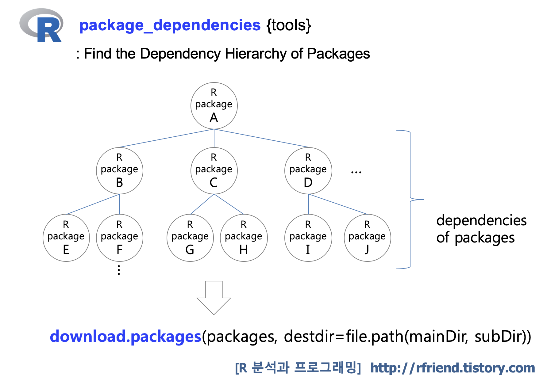
> packages <- getPackages(c("dplyr", "ggplot2"))

download.packages(packages, destdir=file.path(mainDir, subDir))


trying URL 'https://cran.rstudio.com/src/contrib/dplyr_0.8.0.1.tar.gz'

Content type 'application/x-gzip' length 1075146 bytes (1.0 MB)

==================================================

downloaded 1.0 MB

trying URL 'https://cran.rstudio.com/src/contrib/ggplot2_3.1.1.tar.gz'

Content type 'application/x-gzip' length 2862022 bytes (2.7 MB)

==================================================

downloaded 2.7 MB

trying URL 'https://cran.rstudio.com/src/contrib/assertthat_0.2.1.tar.gz'

Content type 'application/x-gzip' length 12742 bytes (12 KB)

==================================================

downloaded 12 KB

trying URL 'https://cran.rstudio.com/src/contrib/glue_1.3.1.tar.gz'

Content type 'application/x-gzip' length 122950 bytes (120 KB)

==================================================

downloaded 120 KB

trying URL 'https://cran.rstudio.com/src/contrib/magrittr_1.5.tar.gz'

Content type 'application/x-gzip' length 200504 bytes (195 KB)

==================================================

downloaded 195 KB

Warning in download.packages(packages, destdir = file.path(mainDir, subDir)) :

  no package 'methods' at the repositories

trying URL 'https://cran.rstudio.com/src/contrib/pkgconfig_2.0.2.tar.gz'

Content type 'application/x-gzip' length 6024 bytes

==================================================

downloaded 6024 bytes

trying URL 'https://cran.rstudio.com/src/contrib/R6_2.4.0.tar.gz'

Content type 'application/x-gzip' length 31545 bytes (30 KB)

==================================================

downloaded 30 KB

trying URL 'https://cran.rstudio.com/src/contrib/Rcpp_1.0.1.tar.gz'

Content type 'application/x-gzip' length 3661123 bytes (3.5 MB)

==================================================

downloaded 3.5 MB

trying URL 'https://cran.rstudio.com/src/contrib/rlang_0.3.4.tar.gz'

Content type 'application/x-gzip' length 858992 bytes (838 KB)

==================================================

downloaded 838 KB

trying URL 'https://cran.rstudio.com/src/contrib/tibble_2.1.1.tar.gz'

Content type 'application/x-gzip' length 311836 bytes (304 KB)

==================================================

downloaded 304 KB

trying URL 'https://cran.rstudio.com/src/contrib/tidyselect_0.2.5.tar.gz'

Content type 'application/x-gzip' length 21883 bytes (21 KB)

==================================================

downloaded 21 KB

Warning in download.packages(packages, destdir = file.path(mainDir, subDir)) :

  no package 'utils' at the repositories

Warning in download.packages(packages, destdir = file.path(mainDir, subDir)) :

  no package 'tools' at the repositories

trying URL 'https://cran.rstudio.com/src/contrib/cli_1.1.0.tar.gz'

Content type 'application/x-gzip' length 40232 bytes (39 KB)

==================================================

downloaded 39 KB

trying URL 'https://cran.rstudio.com/src/contrib/crayon_1.3.4.tar.gz'

Content type 'application/x-gzip' length 658694 bytes (643 KB)

==================================================

downloaded 643 KB

trying URL 'https://cran.rstudio.com/src/contrib/fansi_0.4.0.tar.gz'

Content type 'application/x-gzip' length 266123 bytes (259 KB)

==================================================

downloaded 259 KB

trying URL 'https://cran.rstudio.com/src/contrib/pillar_1.3.1.tar.gz'

Content type 'application/x-gzip' length 103972 bytes (101 KB)

==================================================

downloaded 101 KB

trying URL 'https://cran.rstudio.com/src/contrib/purrr_0.3.2.tar.gz'

Content type 'application/x-gzip' length 373701 bytes (364 KB)

==================================================

downloaded 364 KB

Warning in download.packages(packages, destdir = file.path(mainDir, subDir)) :

  no package 'grDevices' at the repositories

trying URL 'https://cran.rstudio.com/src/contrib/utf8_1.1.4.tar.gz'

Content type 'application/x-gzip' length 218882 bytes (213 KB)

==================================================

downloaded 213 KB

trying URL 'https://cran.rstudio.com/src/contrib/digest_0.6.18.tar.gz'

Content type 'application/x-gzip' length 128553 bytes (125 KB)

==================================================

downloaded 125 KB

Warning in download.packages(packages, destdir = file.path(mainDir, subDir)) :

  no package 'grid' at the repositories

trying URL 'https://cran.rstudio.com/src/contrib/gtable_0.3.0.tar.gz'

Content type 'application/x-gzip' length 368081 bytes (359 KB)

==================================================

downloaded 359 KB

trying URL 'https://cran.rstudio.com/src/contrib/lazyeval_0.2.2.tar.gz'

Content type 'application/x-gzip' length 83482 bytes (81 KB)

==================================================

downloaded 81 KB

trying URL 'https://cran.rstudio.com/src/contrib/MASS_7.3-51.4.tar.gz'

Content type 'application/x-gzip' length 487233 bytes (475 KB)

==================================================

downloaded 475 KB

trying URL 'https://cran.rstudio.com/src/contrib/mgcv_1.8-28.tar.gz'

Content type 'application/x-gzip' length 915991 bytes (894 KB)

==================================================

downloaded 894 KB

trying URL 'https://cran.rstudio.com/src/contrib/plyr_1.8.4.tar.gz'

Content type 'application/x-gzip' length 392451 bytes (383 KB)

==================================================

downloaded 383 KB

trying URL 'https://cran.rstudio.com/src/contrib/reshape2_1.4.3.tar.gz'

Content type 'application/x-gzip' length 36405 bytes (35 KB)

==================================================

downloaded 35 KB

trying URL 'https://cran.rstudio.com/src/contrib/scales_1.0.0.tar.gz'

Content type 'application/x-gzip' length 299262 bytes (292 KB)

==================================================

downloaded 292 KB

Warning in download.packages(packages, destdir = file.path(mainDir, subDir)) :

  no package 'stats' at the repositories

trying URL 'https://cran.rstudio.com/src/contrib/viridisLite_0.3.0.tar.gz'

Content type 'application/x-gzip' length 44019 bytes (42 KB)

==================================================

downloaded 42 KB

trying URL 'https://cran.rstudio.com/src/contrib/withr_2.1.2.tar.gz'

Content type 'application/x-gzip' length 53578 bytes (52 KB)

==================================================

downloaded 52 KB

Warning in download.packages(packages, destdir = file.path(mainDir, subDir)) :

  no package 'graphics' at the repositories

trying URL 'https://cran.rstudio.com/src/contrib/nlme_3.1-139.tar.gz'

Content type 'application/x-gzip' length 793473 bytes (774 KB)

==================================================

downloaded 774 KB

trying URL 'https://cran.rstudio.com/src/contrib/Matrix_1.2-17.tar.gz'

Content type 'application/x-gzip' length 1860456 bytes (1.8 MB)

==================================================

downloaded 1.8 MB

Warning in download.packages(packages, destdir = file.path(mainDir, subDir)) :

  no package 'splines' at the repositories

trying URL 'https://cran.rstudio.com/src/contrib/stringr_1.4.0.tar.gz'

Content type 'application/x-gzip' length 135777 bytes (132 KB)

==================================================

downloaded 132 KB

trying URL 'https://cran.rstudio.com/src/contrib/labeling_0.3.tar.gz'

Content type 'application/x-gzip' length 10722 bytes (10 KB)

==================================================

downloaded 10 KB

trying URL 'https://cran.rstudio.com/src/contrib/munsell_0.5.0.tar.gz'

Content type 'application/x-gzip' length 182653 bytes (178 KB)

==================================================

downloaded 178 KB

trying URL 'https://cran.rstudio.com/src/contrib/RColorBrewer_1.1-2.tar.gz'

Content type 'application/x-gzip' length 11532 bytes (11 KB)

==================================================

downloaded 11 KB

trying URL 'https://cran.rstudio.com/src/contrib/lattice_0.20-38.tar.gz'

Content type 'application/x-gzip' length 359031 bytes (350 KB)

==================================================

downloaded 350 KB

trying URL 'https://cran.rstudio.com/src/contrib/colorspace_1.4-1.tar.gz'

Content type 'application/x-gzip' length 2152594 bytes (2.1 MB)

==================================================

downloaded 2.1 MB

trying URL 'https://cran.rstudio.com/src/contrib/stringi_1.4.3.tar.gz'

Content type 'application/x-gzip' length 7290890 bytes (7.0 MB)

==================================================

downloaded 7.0 MB

      [,1]           [,2]                                                       

 [1,] "dplyr"        "/Users/ihongdon/Downloads/r-pkg/dplyr_0.8.0.1.tar.gz"     

 [2,] "ggplot2"      "/Users/ihongdon/Downloads/r-pkg/ggplot2_3.1.1.tar.gz"     

 [3,] "assertthat"   "/Users/ihongdon/Downloads/r-pkg/assertthat_0.2.1.tar.gz"  

 [4,] "glue"         "/Users/ihongdon/Downloads/r-pkg/glue_1.3.1.tar.gz"        

 [5,] "magrittr"     "/Users/ihongdon/Downloads/r-pkg/magrittr_1.5.tar.gz"      

 [6,] "pkgconfig"    "/Users/ihongdon/Downloads/r-pkg/pkgconfig_2.0.2.tar.gz"   

 [7,] "R6"           "/Users/ihongdon/Downloads/r-pkg/R6_2.4.0.tar.gz"          

 [8,] "Rcpp"         "/Users/ihongdon/Downloads/r-pkg/Rcpp_1.0.1.tar.gz"        

 [9,] "rlang"        "/Users/ihongdon/Downloads/r-pkg/rlang_0.3.4.tar.gz"       

[10,] "tibble"       "/Users/ihongdon/Downloads/r-pkg/tibble_2.1.1.tar.gz"      

[11,] "tidyselect"   "/Users/ihongdon/Downloads/r-pkg/tidyselect_0.2.5.tar.gz"  

[12,] "cli"          "/Users/ihongdon/Downloads/r-pkg/cli_1.1.0.tar.gz"         

[13,] "crayon"       "/Users/ihongdon/Downloads/r-pkg/crayon_1.3.4.tar.gz"      

[14,] "fansi"        "/Users/ihongdon/Downloads/r-pkg/fansi_0.4.0.tar.gz"       

[15,] "pillar"       "/Users/ihongdon/Downloads/r-pkg/pillar_1.3.1.tar.gz"      

[16,] "purrr"        "/Users/ihongdon/Downloads/r-pkg/purrr_0.3.2.tar.gz"       

[17,] "utf8"         "/Users/ihongdon/Downloads/r-pkg/utf8_1.1.4.tar.gz"        

[18,] "digest"       "/Users/ihongdon/Downloads/r-pkg/digest_0.6.18.tar.gz"     

[19,] "gtable"       "/Users/ihongdon/Downloads/r-pkg/gtable_0.3.0.tar.gz"      

[20,] "lazyeval"     "/Users/ihongdon/Downloads/r-pkg/lazyeval_0.2.2.tar.gz"    

[21,] "MASS"         "/Users/ihongdon/Downloads/r-pkg/MASS_7.3-51.4.tar.gz"     

[22,] "mgcv"         "/Users/ihongdon/Downloads/r-pkg/mgcv_1.8-28.tar.gz"       

[23,] "plyr"         "/Users/ihongdon/Downloads/r-pkg/plyr_1.8.4.tar.gz"        

[24,] "reshape2"     "/Users/ihongdon/Downloads/r-pkg/reshape2_1.4.3.tar.gz"    

[25,] "scales"       "/Users/ihongdon/Downloads/r-pkg/scales_1.0.0.tar.gz"      

[26,] "viridisLite"  "/Users/ihongdon/Downloads/r-pkg/viridisLite_0.3.0.tar.gz

[27,] "withr"        "/Users/ihongdon/Downloads/r-pkg/withr_2.1.2.tar.gz"       

[28,] "nlme"         "/Users/ihongdon/Downloads/r-pkg/nlme_3.1-139.tar.gz"      

[29,] "Matrix"       "/Users/ihongdon/Downloads/r-pkg/Matrix_1.2-17.tar.gz"     

[30,] "stringr"      "/Users/ihongdon/Downloads/r-pkg/stringr_1.4.0.tar.gz"     

[31,] "labeling"     "/Users/ihongdon/Downloads/r-pkg/labeling_0.3.tar.gz"      

[32,] "munsell"      "/Users/ihongdon/Downloads/r-pkg/munsell_0.5.0.tar.gz"     

[33,] "RColorBrewer" "/Users/ihongdon/Downloads/r-pkg/RColorBrewer_1.1-2.tar.gz"

[34,] "lattice"      "/Users/ihongdon/Downloads/r-pkg/lattice_0.20-38.tar.gz"   

[35,] "colorspace"   "/Users/ihongdon/Downloads/r-pkg/colorspace_1.4-1.tar.gz"  

[36,] "stringi"      "/Users/ihongdon/Downloads/r-pkg/stringi_1.4.3.tar.gz"


위에 다운로드된 패키지들의 리스트를 보면 알 수 있는 것처럼, 'dplyr'과 'ggplot2'의 두 개 패키지를 다운로드 하려고 했더니 이들이 의존성을 가지고 있는 [3] 'assertthat' 패키지부터 ~ [36] 'stringi' 패키지까지 34개의 패키지가 추가로 다운로드 되었습니다. 


외부의 인터넷 연결이 되는 환경에서 다운받아 놓은 이들 R packages 파일들을 저장매체에 저장하여 가져가서 폐쇄망으로 되어 있는 서버에 복사를 한 후에, 수작업으로 R package 설치하면 되겠습니다. (이때 의존성 있는 패키지들까지 알아서 다 설치가 되도록 여러번 설치 작업을 반복해주면 됩니다. 


아래 코드를 사용하시면 다운로드 받아놓은 모든 패키지의 리스트를 읽어와서 수동으로 R 패키지 설치를 할 수 있습니다. 


## set working directory
setwd("C:/Users/hdlee/Documents/R") # set with yours

## getting the list of R packages downloaded
src_pkgs <- list.files("C:/Users/hdlee/Documents/R") # use yours

## install R packages manually using binary files
install.packages(src_pkgs, repos = NULL, type = "source")


##==============================================##

폐쇄망 환경에서 Greenplum DB에 R 패키지 설치하는 방법은 

== > http://gpdbkr.blogspot.com/2019/12/greenplum-6-plr-r.html

==> https://rfriend.tistory.com/442 

포스팅을 참고하세요. 

##==============================================##


많은 도움이 되었기를 바랍니다. 

728x90
반응형
Posted by Rfriend
,

이번 포스팅에서는 행 기준으로 숫자형 변수들의 합을 구한 다음에, 그룹별로 행 기준 합이 최대인 전체 행을 선별하는 방법을 소개하겠습니다. 


말로 설명한 내용만으로는 얼른 이해가 안 올 수도 있겠는데요, 이번에 해볼 내용은 아래의 이미지를 참고하시면 이해가 쉬울 듯 합니다. 


예제로 사용할 하나의 그룹 변수(V1)와 나머지 9개의 숫자형 변수(V2~V10)로 구성된 간단한 DataFrame을 만들어보겠습니다. 


> ##------------------------------------------------------

> ## selecting distinct object using dplyr chain operator

> ##------------------------------------------------------

> rm(list=ls())

> set.seed(123) # for reproducibility

> V1 <- c(rep("apple", 5), rep("banana", 5), rep("tomato", 5)) # group

> V2 <- sample(x=1:10, size=15, replace=T)

> V3 <- sample(x=1:10, size=15, replace=T)

> V4 <- sample(x=1:10, size=15, replace=T)

> V5 <- sample(x=1:10, size=15, replace=T)

> V6 <- sample(x=1:10, size=15, replace=T)

> V7 <- sample(x=1:10, size=15, replace=T)

> V8 <- sample(x=1:10, size=15, replace=T)

> V9 <- sample(x=1:10, size=15, replace=T)

> V10 <- sample(x=1:10, size=15, replace=T)

> df <- data.frame(V1, V2, V3, V4, V5, V6, V7, V8, V9, V10)

> df

       V1 V2 V3 V4 V5 V6 V7 V8 V9 V10

1   apple  3  9 10  2  7  3  2  9   7

2   apple  8  3 10  3  1  4  7 10   4

3   apple  5  1  7  5  4  7  4  7   4

4   apple  9  4  8  3  3  4  7  5   3

5   apple 10 10  1  9  9  2  4  2   4

6  banana  1  9  5  1  5  3  2 10  10

7  banana  6  7  8  5  9  7  8  4   2

8  banana  9  7  3  8  9  5  1  1   1

9  banana  6 10  4  2  8  8  5 10   2

10 banana  5  7  3  6  5  2  6  8   7

11 tomato 10  8  2  3  8  5  6  2   7

12 tomato  5  6  5  2  7 10  4  6   9

13 tomato  7  6  5  8  8  9  5 10   7

14 tomato  6  3  4  9  1  9 10  6   8

15 tomato  2  2  2  4  5  2  5  5   6


> rm(V1, V2, V3, V4, V5, V6, V7, V8, V9, V10)


rowSums() 함수를 사용하여서 행(row) 기준의 숫자형 변수들 모두에 대해 합계를 구하여 'V_sum' 이라는 새로운 변수를 추가해보겠습니다. 


> # summation in a row direction

> df$V_sum <- rowSums(df[,2:10])

> df

       V1 V2 V3 V4 V5 V6 V7 V8 V9 V10 V_sum


1   apple  3  9 10  2  7  3  2  9   7    52

2   apple  8  3 10  3  1  4  7 10   4    50

3   apple  5  1  7  5  4  7  4  7   4    44

4   apple  9  4  8  3  3  4  7  5   3    46

5   apple 10 10  1  9  9  2  4  2   4    51


6  banana  1  9  5  1  5  3  2 10  10    46

7  banana  6  7  8  5  9  7  8  4   2    56

8  banana  9  7  3  8  9  5  1  1   1    44

9  banana  6 10  4  2  8  8  5 10   2    55

10 banana  5  7  3  6  5  2  6  8   7    49


11 tomato 10  8  2  3  8  5  6  2   7    51

12 tomato  5  6  5  2  7 10  4  6   9    54

13 tomato  7  6  5  8  8  9  5 10   7    65

14 tomato  6  3  4  9  1  9 10  6   8    56

15 tomato  2  2  2  4  5  2  5  5   6    33


위의 행 기준 합계로 보면 'apple' 그룹에서는 1번째 행의 합이 52로 가장 크며, 'banana' 그룹에서는 7번째 행의 합이 56으로서 가장 크고, 'tomato' 그룹에서는 13번째 행의 합이 65로서 가장 큽니다. 이를 1번째, 7번째, 13번째 전체 행을 선별해보겠습니다. (빨간색으로 표시한 부분)


> library(dplyr)

> df_group_distinct_max <- df %>% 

+   arrange(V1, desc(V_sum)) %>% 

+   group_by(V1) %>% slice(1:1)

> df_group_distinct_max <- data.frame(df_group_distinct_max[1:10])

> df_group_distinct_max

      V1 V2 V3 V4 V5 V6 V7 V8 V9 V10

1  apple  3  9 10  2  7  3  2  9   7

2 banana  6  7  8  5  9  7  8  4   2

3 tomato  7  6  5  8  8  9  5 10   7


* dplyr 패키지 사용법은 

https://rfriend.tistory.com/234 , 

https://rfriend.tistory.com/236

참고하시기 바랍니다


많은 도움이 되었기를 바랍니다. 


이번 포스팅이 도움이 되었다면 아래의 '공감~'를 꾹 눌러주세요. ^^


728x90
반응형
Posted by Rfriend
,