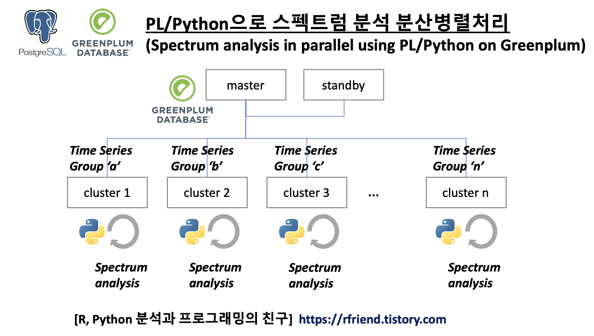
이전 포스팅에서 스펙트럼 분석(spectrum analysis, spectral analysis, frequency domain analysis) 에 대해서 소개하였습니다. ==> https://rfriend.tistory.com/690 참조
이번 포스팅에서는 Greenplum 에서 PL/Python (Procedural Language)을 활용하여 여러개 그룹의 시계열 데이터에 대해 스펙트럼 분석을 분산병렬처리하는 방법을 소개하겠습니다. (spectrum analysis in parallel using PL/Python on Greenplum database)
spectrum analysis in parallel using PL/Python on Greenplum
(1) 다른 주파수를 가진 3개 그룹의 샘플 데이터셋 생성
먼저, spectrum 모듈에서 data_cosine() 메소드를 사용하여 주파수(frequency)가 100, 200, 250 인 3개 그룹의 코사인 파동 샘플 데이터를 생성해보겠습니다. (노이즈 A=0.1 만큼이 추가된 1,024개 코사인 데이터 포인트를 가진 예제 데이터)
## generating 3 cosine signals with frequency of (100Hz, 200Hz, 250Hz) respectively
## buried in white noise (amplitude 0.1), a length of N=1024 and the sampling is 1024Hz.
from spectrum import data_cosine

data1 = data_cosine(N=1024, A=0.1, sampling=1024, freq=100)
data2 = data_cosine(N=1024, A=0.1, sampling=1024, freq=200)
data3 = data_cosine(N=1024, A=0.1, sampling=1024, freq=250)
다음으로 Python pandas 모듈을 사용해서 'grp' 라는 칼럼에 'a', 'b', 'c'의 구분자를 추가하고, 'val' 칼럼에는 위에서 생성한 각기 다른 주파수를 가지는 3개의 샘플 데이터셋을 값으로 가지는 DataFrame을 생성합니다.
## making a pandas DataFrame with a group name
import pandas as pd

df1 = pd.DataFrame({'grp': 'a', 'val': data1})
df2 = pd.DataFrame({'grp': 'b', 'val': data2})
df3 = pd.DataFrame({'grp': 'c', 'val': data3})

df = pd.concat([df1, df2, df3])


df.shape
# (3072, 2)


df.head()
# 	grp	val
# 0	a	1.056002
# 1	a	0.863020
# 2	a	0.463375
# 3	a	-0.311347
# 4	a	-0.756723
sqlalchemy 모듈의 create_engine("driver://user:password@host:port/database") 메소드를 사용해서 Greenplum 데이터베이스에 접속한 후에 pandas의 DataFrame.to_sql() 메소드를 사용해서 위에서 만든 pandas DataFrame을 Greenplum DB에 import 하도록 하겠습니다.
이때 index = True, indx_label = 'id' 를 꼭 설정해주어야만 합니다. 그렇지 않을 경우 Greenplum DB에 데이터가 import 될 때 시계열 데이터의 특성이 sequence 가 없이 순서가 뒤죽박죽이 되어서, 이후에 스펙트럼 분석을 할 수 없게 됩니다.
## importing data to Greenplum using pandas
import sqlalchemy
from sqlalchemy import create_engine

# engine = sqlalchemy.create_engine("postgresql://user:password@host:port/database")
engine = create_engine("postgresql://user:password@ip:5432/database") # set with yours

df.to_sql(name = 'data_cosine',
          con = engine,
          schema = 'public',
          if_exists = 'replace', # {'fail', 'replace', 'append'), default to 'fail'
          index = True,
          index_label = 'id',
          chunksize = 100,
          dtype = {
              'id': sqlalchemy.types.INTEGER(),
              'grp': sqlalchemy.types.TEXT(),
              'val': sqlalchemy.types.Float(precision=6)
          })


SELECT * FROM data_cosine order by grp, id LIMIT 5;
# id	grp	val
# 0	a	1.056
# 1	a	0.86302
# 2	a	0.463375
# 3	a	-0.311347
# 4	a	-0.756723


SELECT count(1) AS cnt FROM data_cosine;
# cnt
# 3072
(2) 스펙트럼 분석을 분산병렬처리하는 PL/Python 사용자 정의 함수 정의 (UDF definition)
아래의 스펙트럼 분석은 Python scipy 모듈의 signal() 메소드를 사용하였습니다. (spectrum 모듈의 Periodogram() 메소드를 사용해도 동일합니다. https://rfriend.tistory.com/690 참조)
(Greenplum database의 master node와 segment nodes 에는 numpy와 scipy 모듈이 각각 미리 설치되어 있어야 합니다.)
사용자 정의함수의 인풋으로는 (a) 시계열 데이터 array 와 (b) sampling frequency 를 받으며, 아웃풋으로는 스펙트럼 분석을 통해 추출한 주파수(frequency, spectrum)를 텍스트(혹은 int)로 반환하도록 하였습니다.
DROP FUNCTION IF EXISTS spectrum_func(float8[], int);
CREATE OR REPLACE FUNCTION spectrum_func(x float8[], fs int)
RETURNS text
AS $$
    from scipy import signal
    import numpy as np

    # x: Time series of measurement values
    # fs: Sampling frequency of the x time series. Defaults to 1.0.
    f, PSD = signal.periodogram(x, fs=fs)
    freq = np.argmax(PSD)

    return freq

$$ LANGUAGE 'plpythonu';
(3) 스펙트럼 분석을 분산병렬처리하는 PL/Python 사용자 정의함수 실행 (Execution of Spectrum Analysis in parallel on Greenplum)
위의 (2)번에서 정의한 스펙트럼 분석 PL/Python 사용자 정의함수 spectrum_func(x, fs) 를 Select 문으로 호출하여 실행합니다. FROM 절에는 sub query로 input에 해당하는 시계열 데이터를 ARRAY_AGG() 함수를 사용해 array 로 묶어주는데요, 이때 ARRAY_AGG(val::float8 ORDER BY id) 로 id 기준으로 반드시 시간의 순서에 맞게 정렬을 해주어야 제대로 스펙트럼 분석이 진행이 됩니다.
SELECT
    grp
    , spectrum_func(val_agg, 1024)::int AS freq
FROM (
    SELECT
        grp
        , ARRAY_AGG(val::float8 ORDER BY id) AS val_agg
    FROM data_cosine
    GROUP BY grp
) a
ORDER BY grp;

# grp	freq
# a	100
# b	200
# c	250
우리가 (1)번에서 주파수가 각 100, 200, 250인 샘플 데이터셋을 만들었는데요, 스펙트럼 분석을 해보니 정확하게 주파수를 도출해 내었네요!.
Database에서 가상의 샘플 데이터를 만들어서 SQL이 버그없이 잘 작동하는지 확인을 한다든지, DB의 성능을 테스트 해봐야 할 때가 있습니다.
이번 포스팅에서는 PostgreSQL, Greenplum DB를 사용해서 정규분포(Normal Distribution)로부터 난수 (random number)를 생성하여 샘플 테이블을 만들어보겠습니다.
(1) 테이블 생성 : create table
(2) 정규분포로 부터 난수 생성하는 사용자 정의 함수 정의 : random_normal(count, mean, stddev)
(3) 테이블에 정규분포로 부터 생성한 난수 추가하기 : generate_series(), to_char(), insert into
(4) Instance 별 데이터 개수 확인하기 : count() group by gp_segment_id
creating a sample table using random numbers in PostgreSQL, Greenplum
아래 SQL 예제 코드는 PostgreSQL 9.4.26 버전, Greenplum 6.19.2 버전에서, Greenplum Database 의 분산 저장, 분산병렬처리 고려해서 작성하였습니다.
-- version check
SELECT version();
-- PostgreSQL 9.4.26 (Greenplum Database 6.19.2 build commit:0e1f6307eb4e368b79cbf67a0dc6af53362d26c0) on x86_64-unknown-linux-gnu, compiled by gcc (GCC) 6.4.0, 64-bit compiled on Feb 14 2022 23:03:52
(1) 테이블 생성 : create table
CREATE TABLE 함수를 사용해서 분석의 대상 기준으로 사용할 문자열의 cell_id, param_id 와 숫자형의 측정값 meas_val 을 가지는 빈 껍데기 samp_tbl 테이블을 만들어보겠습니다. WITH 절에 압축 옵션을 설정하였으며, DISTRIBUTED BY (cell_id) 로 분산 저장하는 기준을 설정해주었습니다.
분산키를 잘 잡아주는 것이 향후 분산병렬처리의 성능을 좌지우지 합니다. 분석이나 데이터 처리(조인 등) 기준이 되고, 한쪽 노드로 쏠리지 않고 골고루 분산시킬 수 있는 분산키를 설정해주어야 합니다.
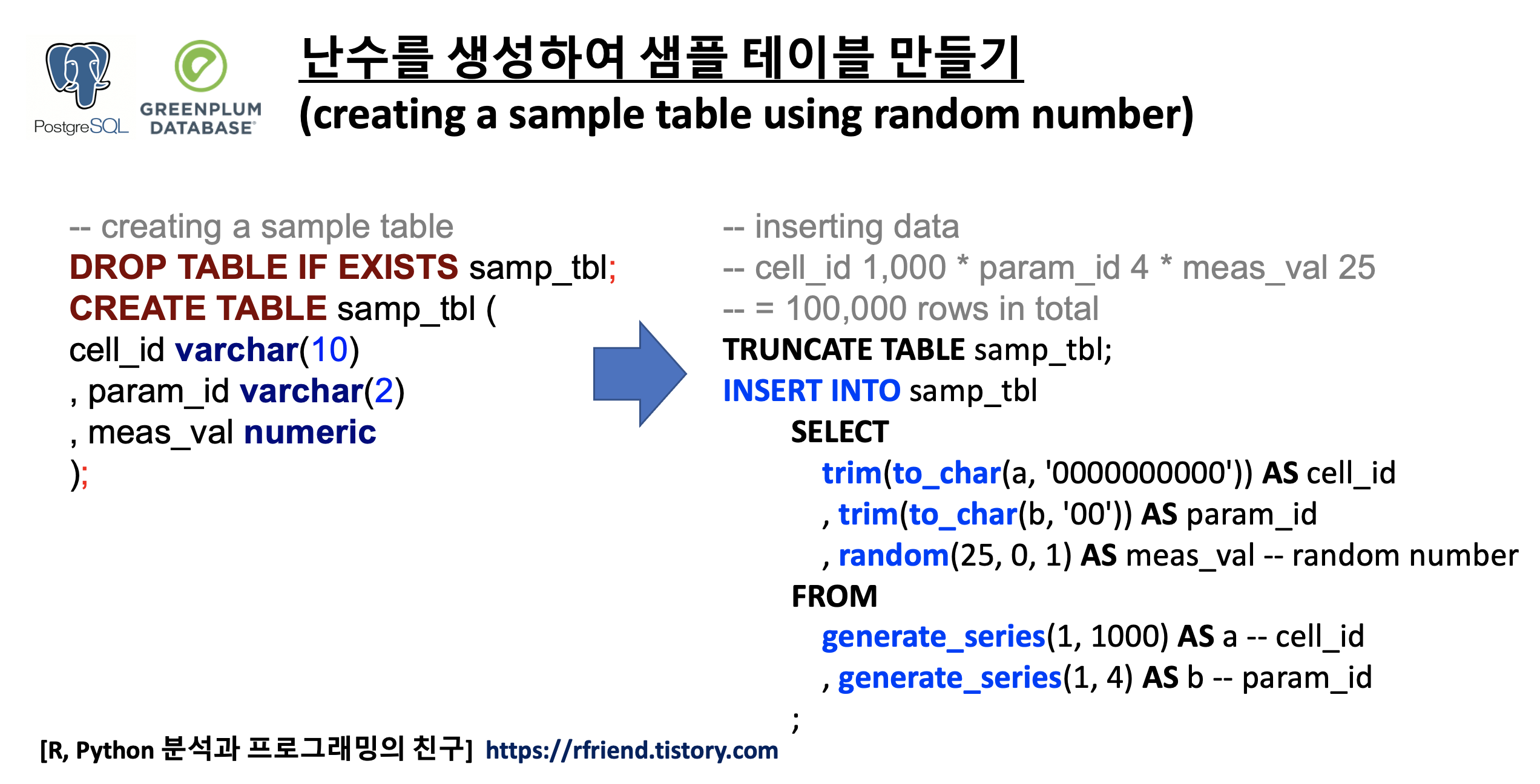
-- creating a sample table
DROP TABLE IF EXISTS samp_tbl;
CREATE TABLE samp_tbl (
	cell_id varchar(10)
	, param_id varchar(2)
	, meas_val numeric
) WITH(appendonly=TRUE, compresslevel=7, compresstype=zstd)
DISTRIBUTED BY (cell_id);
(2) 정규분포로 부터 난수 생성하는 사용자 정의 함수 정의 : random_normal(count, mean, stddev)
PostgreSQL 버전 10 이상부터 정규분포(normal distribution)로 부터 난수를 생성(generating random numbers) 하는 함수 normal_rand() 를 쓸 수 있습니다.
-- over PostgreSQL version 10
-- Produces a set of normally distributed random values.
normal_rand ( numvals integer, mean float8, stddev float8 ) → setof float8
PostgreSQL 9.6 이전 버전에서는PL/Python, PL/R, PL/SQL 로 정규분포로 부터 난수를 생성하는 사용자 정의함수를 정의해서 사용해야 합니다. (아래는 PL/SQL 이구요, PL/Python이나 PL/R 로도 가능해요)
-- UDF of random number generator from a normal distribution, X~N(mean, stddev)
-- random_normal() built-in function over PostgreSQL version 10.x
DROP FUNCTION IF EXISTS random_normal(INTEGER, DOUBLE PRECISION, DOUBLE PRECISION);
CREATE OR REPLACE FUNCTION random_normal(
    count INTEGER DEFAULT 1,
    mean DOUBLE PRECISION DEFAULT 0.0,
    stddev DOUBLE PRECISION DEFAULT 1.0
    ) RETURNS SETOF DOUBLE PRECISION
      RETURNS NULL ON NULL INPUT AS $$
        DECLARE
            u DOUBLE PRECISION;
            v DOUBLE PRECISION;
            s DOUBLE PRECISION;
        BEGIN
            WHILE count > 0 LOOP
                u = RANDOM() * 2 - 1; -- range: -1.0 <= u < 1.0
                v = RANDOM() * 2 - 1; -- range: -1.0 <= v < 1.0
                s = u^2 + v^2;

                IF s != 0.0 AND s < 1.0 THEN
                    s = SQRT(-2 * LN(s) / s);

                    RETURN NEXT mean + stddev * s * u;
                    count = count - 1;

                    IF count > 0 THEN
                        RETURN NEXT mean + stddev * s * v;
                        count = count - 1;
                    END IF;
                END IF;
            END LOOP;
        END;
    $$ LANGUAGE plpgsql;


    -- credit: https://bugfactory.io/blog/generating-random-numbers-according-to-a-continuous-probability-distribution-with-postgresql/
(3) 테이블에 정규분포로 부터 생성한 난수 추가하기 : generate_series(), to_char(), insert into
이제 위의 (1)번에서 생성한 samp_tbl 테이블에 insert into 구문을 사용해서 가상의 샘플 데이터 추가해보겠습니다. 이때 From 절에서 generate_series(from, to) 함수를 사용해서 정수의 수열을 생성해주고, SELECT 절의 TO_CHAR(a, '0000000000'), TO_CHAR(b, '00') 에서 generate_series()에서 생성한 정수를자리수가 10자리, 2자리인 문자열로 바꾸어줍니다. (빈 자리는 '0'으로 자리수만큼 채워줍니다.) TRIP() 함수는 화이트 스페이스를 제거해줍니다.
-- inserting data
-- cell_id 1,000 * param_id 4 * meas_val 25 = 100,000 rows in total
-- good cases 99,999,000 vs. bad cases 1,000 (cell_id 10 * param_id 4 * meas_val 25 = 1,000 rows)
-- cell_id '000000001' will be used as a control group (good case) later.
-- it took 8 min. 4 sec.
TRUNCATE TABLE samp_tbl;
INSERT INTO samp_tbl
SELECT
	trim(to_char(a, '0000000000')) AS cell_id
	, trim(to_char(b, '00')) AS param_id
	, random_normal(25, 0, 1) AS meas_val -- X~N(0, 1), from Normal distribution
FROM generate_series(1, 1000) AS a -- cell_id
	, generate_series(1, 4) AS b -- param_id
;
(4) Instance 별 데이터 개수 확인하기 : count() group by gp_segment_id
위의 (1)~(3)번에서 테이블을 만들고, 가짜 데이터를 정규분포로 부터 난수를 발생시켜서 테이블에 추가를 하였으니, Greenplum의 각 nodes 에 골고루 잘 분산이 되었는지 확인을 해보겠습니다. (아래는 AWS에서 2개 노드, 노드별 6개 instance, 총 12개 instances 환경에서 테스트한 것임)
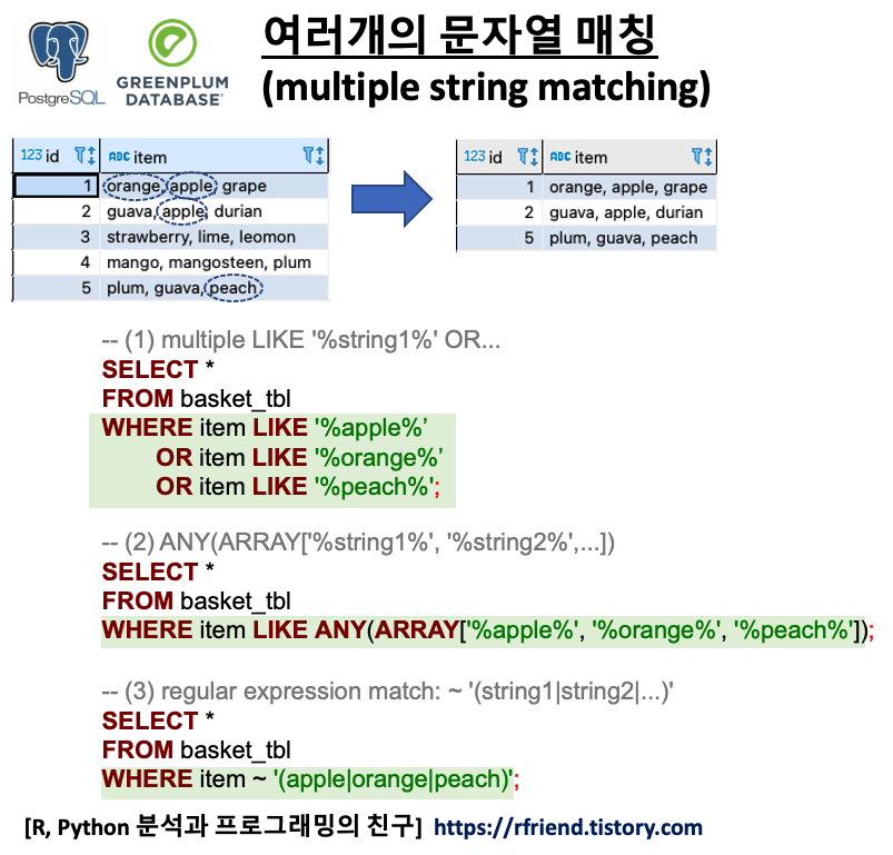
먼저 예제로 사용할 샘플 테이블을 만들어보겠습니다. 과일가게에서 장바구니 ID별로 구매한 과일 품목이 문자열로 들어있는 테이블입니다.
-- create a sample table
DROP TABLE IF EXISTS basket_tbl;
CREATE TABLE basket_tbl (
	id int
	, item text
);


INSERT INTO basket_tbl VALUES
(1, 'orange, apple, grape')
, (2, 'guava, apple, durian')
, (3, 'strawberry, lime, leomon')
, (4, 'mango, mangosteen, plum')
, (5, 'plum, guava, peach');

SELECT * FROM basket_tbl ORDER BY id;
--id|item                    |
----+------------------------+
-- 1|orange, apple, grape    |
-- 2|guava, apple, durian    |
-- 3|strawberry, lime, leomon|
-- 4|mango, mangosteen, plum |
-- 5|plum, guava, peach      |
위의 샘플 테이블의 item 칼럼의 문자열에서 'apple', 'orange', 'peach' 중에 하나라도(OR) 문자열이 매칭(string matching)이 되면 SELECT 문으로 조회를 해오는 SQL query 를 3가지 방법으로 작성해보겠습니다.
(1) LIKE '%string1%' OR LIKE '%string2%' ...
가장 단순한 반면에, 조건절 항목이 많아질 경우 SQL query 가 굉장히 길어지고 비효율적인 단점이 있습니다.
-- (1) multiple LIKE '%string1%' OR LIKE '%string2%' OR...
SELECT *
FROM basket_tbl
WHERE item LIKE '%apple%'
	OR item LIKE '%orange%'
	OR item LIKE '%peach%'
ORDER BY id;

--id|item                |
----+--------------------+
-- 1|orange, apple, grape|
-- 2|guava, apple, durian|
-- 5|plum, guava, peach  |
(2) ANY(ARRAY['%string1%', '%string2%', ...])
문자열 매칭 조건절의 각 문자열 항목을 ARRAY[] 에 나열을 해주고, any() 연산자를 사용해서 이들 문자열 조건 중에서 하나라도 매칭이 되면 반환을 하도록 하는 방법입니다. 위의 (1)번 보다는 SQL query 가 짧고 깔끔해졌습니다.
-- (2) ANY(ARRAY['%string1%', '%string2%',...])
SELECT *
FROM basket_tbl
WHERE item LIKE ANY(ARRAY['%apple%', '%orange%', '%peach%'])
ORDER BY id;

--id|item                |
----+--------------------+
-- 1|orange, apple, grape|
-- 2|guava, apple, durian|
-- 5|plum, guava, peach  |
이번 포스팅에서는 PostgreSQL, Greenplum DB의 Window Function 의 함수 특징, 함수별 구문 사용법에 대해서 알아보겠습니다. Window Function을 알아두면 편리하고 또 강력한 SQL query 를 사용할 수 있습니다. 특히 MPP (Massively Parallel Processing) Architecture 의 Greenplum DB 에서는 Window Function 실행 시 분산병렬처리가 되기 때문에 성능 면에서 매우 우수합니다.
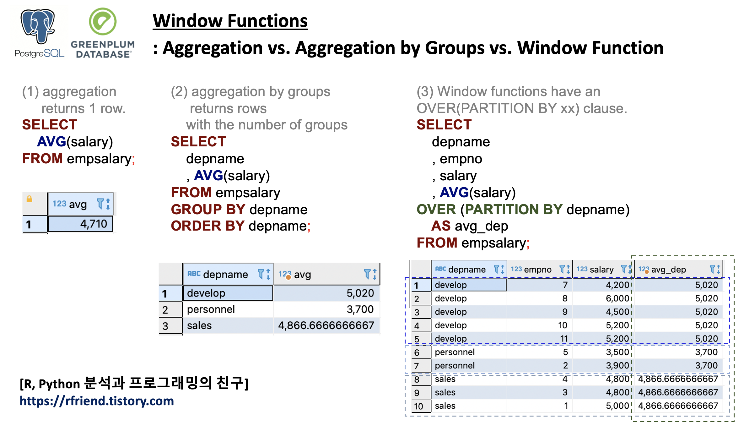
Window Function 은 현재 행과 관련된 테이블 행 집합(a set of table rows)에 대해 계산을 수행합니다. 이는 집계 함수(aggregate function)로 수행할 수 있는 계산 유형과 비슷합니다. 그러나 일반적인 집계 함수와 달리 Window Function을 사용하면 행이 단일 출력 행으로 그룹화되지 않으며 행은 별도의 ID를 유지합니다.
아래 화면의 예시는 AVG() 함수로 평균을 구하는데 있어,
(a) 전체 평균 집계: AVG() --> 한 개의 행 반환
(b) 그룹별 평균 집계: AVG() ... GROUP BY --> 그룹의 개수만큼 행 반환
[ PostgreSQL, Greenplum: Aggregation vs. Aggregation by Groups vs. Window Function ]
PostgreSQL, Greenplum: Aggregation vs. Aggregation by Groups vs. Window Function
먼저, 부서(depname), 직원번호(empno), 급여(salary) 의 칼럼을 가지는 간단한 예제 테이블 empsalary 을 만들고 데이터를 입력해보겠습니다.
-- (0) making a sample table as an example
DROP TABLE IF EXISTS empsalary;
CREATE TABLE empsalary (
	depname TEXT
	, empno INT
	, salary INT
);

INSERT INTO empsalary  (depname, empno, salary)
VALUES
('sales', 1, 5000)
, ('personnel', 2, 3900)
, ('sales', 3, 4800)
, ('sales', 4, 4800)
, ('personnel', 5, 3500)
, ('develop', 7, 4200)
, ('develop', 8, 6000)
, ('develop', 9, 4500)
, ('develop', 10, 5200)
, ('develop' , 11, 5200);

SELECT * FROM empsalary ORDER BY  empno LIMIT 2;

--depname  |empno|salary|
-----------+-----+------+
--sales    |    1|  5000|
--personnel|    2|  3900|
(1) AVG() vs. AVG() GROUP BY vs. AVG() OVER (PARTITION BY ORDER BY)
아래는 (a) AVG() 로 전체 급여의 전체 평균 집계, (b) AVG() GROUP BY depname 로 부서 그룹별 평균 집계, (c) AVG() OVER (PARTITION BY depname) 의 Window Function을 사용해서 부서 집합 별 평균을 계산해서 직원번호 ID의 행별로 결과를 반환하는 것을 비교해 본 것입니다. 반환하는 행의 개수, 결과를 유심히 비교해보시면 aggregate function 과 window function 의 차이를 이해하는데 도움이 될거예요.
-- (0) aggregation returns 1 row.
SELECT
	AVG(salary)
FROM empsalary;

--avg                  |
-----------------------+
--4710.0000000000000000|


-- (0) aggregation by groups returns rows with the number of groups
SELECT
	depname
	, AVG(salary)
FROM empsalary
GROUP BY depname
ORDER BY depname;

--depname  |avg                  |
-----------+---------------------+
--develop  |5020.000000000000000
--personnel|3700.000000000000000
--sales    |4866.6666666666666667|


-- (1) Window functions have an OVER(PARTITION BY xx) clause.
-- any function without an OVER clause is not a window function, but rather an aggregate or single-row (scalar) function.
SELECT
	depname
	, empno
	, salary
	, AVG(salary)
		OVER (PARTITION BY depname)
		AS avg_dep
FROM empsalary;

--depname  |empno|salary|avg_dep              |
-----------+-----+------+---------------------+
--develop  |    7|  4200|5020.0000000000000000|
--develop  |    8|  6000|5020.0000000000000000|
--develop  |    9|  4500|5020.0000000000000000|
--develop  |   10|  5200|5020.0000000000000000|
--develop  |   11|  5200|5020.0000000000000000|
--personnel|    5|  3500|3700.0000000000000000|
--personnel|    2|  3900|3700.0000000000000000|
--sales    |    4|  4800|4866.6666666666666667|
--sales    |    3|  4800|4866.6666666666666667|
--sales    |    1|  5000|4866.6666666666666667|
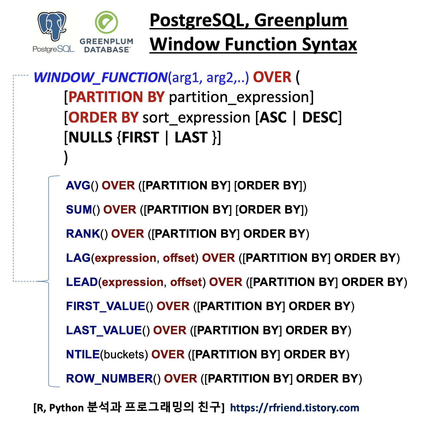
아래는 PostgreSQL, Greenplum 의 Window Function Syntax 구문입니다.
- window_function(매개변수) 바로 다음에 OVER() 가 있으며,
- OVER() 안에 PARTITION BY 로 연산이 실행될 집단(set) 기준을 지정해주고
- OVER() 안에 ORDER BY 로 시간(time), 순서(sequence)가 중요할 경우 정렬 기준을 지정해줍니다.
-- PostgreSQL Window Function Syntax
WINDOW_FUNCTION(arg1, arg2,..) OVER (
	[PARTITION BY partition_expression]
	[ORDER BY sort_expression [ASC | DESC]
	[NULLS {FIRST | LAST }]
	)
PostgreSQL, Greenplum Window Function Syntax
PostgreSQL의 Window Functions 중에서 제가 그래도 자주 쓰는 함수로 AVG() OVER(), SUM() OVER(), RANK() OVER(), LAG() OVER(), LEAD() OVER(), FIRST_VALUE() OVER(), LAST_VALUE() OVER(), NTILE() OVER(), ROW_NUMBER() OVER() 등의 일부 함수 (제 맘대로... ㅎㅎ)에 대해서 아래에 예시를 들어보겠습니다.
(2) RANK() OVER ([PARTITION BY] ORDER BY) : 순위
아래 예는 PARTITION BY depname 로 '부서' 집단별로 구분해서, ORDER BY salary DESC로 급여 내림차순으로 정렬한 후의 직원별 순위(rank)를 계산해서 직원 ID 행별로 순위를 반환해줍니다.
PARTITION BY 집단 내에서 ORDER BY 정렬 기준칼럼의 값이 동일할 경우 순위는 동일한 값을 가지며, 동일한 순위의 개수만큼 감안해서 그 다음 순위의 값은 순위가 바뀝니다. (가령, develop 부서의 경우 순위가 1, 2, 2, 4, 5, 로서 동일 순위 '2'가 두명 있고, 급여가 네번째인 사람의 순위는 '4'가 되었음.)
-- (2) You can control the order
--    in which rows are processed by window functions using ORDER BY within OVER.
SELECT
	depname
	, empno
	, salary
	, RANK() OVER (PARTITION BY depname ORDER BY salary DESC)
FROM empsalary;

--depname  |empno|salary|rank|
-----------+-----+------+----+
--personnel|    2|  3900|   1|
--personnel|    5|  3500|   2|
------------------------------------- set 1 (personnel)
--sales    |    1|  5000|   1|
--sales    |    3|  4800|   2|
--sales    |    4|  4800|   2|
------------------------------------- set 2 (sales)
--develop  |    8|  6000|   1|
--develop  |   11|  5200|   2|
--develop  |   10|  5200|   2|
--develop  |    9|  4500|   4|
--develop  |    7|  4200|   5|
------------------------------------- set 3 (develop)
(3) SUM() OVER () : PARTITION BY, ORDER BY 는 생략 가능
만약 집단별로 구분해서 연산할 필요가 없다면 OVER() 구문 안에서 PARTITON BY 는 생략할 수 있습니다.
만약 시간이나 순서가 중요하지 않다면 OVER() 구문 안에서 ORDER BY 는 생략할 수 있습니다.
아래 예에서는 SUM(salary) OVER () 를 사용해서 전체 직원의 급여 평균을 계산해서 각 직원 ID의 개수 만큼 행을 반환했습니다.
-- (3) ORDER BY can be omitted if the ordering of rows is not important.
-- It is also possible to omit PARTITION BY,
-- in which case there is just one partition containing all the rows.
SELECT
	salary
	, SUM(salary) OVER ()  -- same result
FROM empsalary;

--salary|sum  |
--------+-----+
--  5000|47100|
--  3900|47100|
--  4800|47100|
--  4800|47100|
--  3500|47100|
--  4200|47100|
--  6000|47100|
--  4500|47100|
--  5200|47100|
--  5200|47100|
(4) SUM() OVER (ORDER BY) : ORDER BY 구문이 추가되면 누적 합으로 결과가 달라짐
만약 PARTITION BY 가 없어서 집단별 구분없이 전체 데이터셋을 대상으로 연산을 하게 될 때, SUM(salary) OVER (ORDER BY salary) 처럼 OVER () 절 안에 ORDER BY 를 추가하게 되면 salary 를 기준으로 정렬이 된 상태에서 누적 합이 계산되므로 위의 (3)번과 차이점을 알아두기 바랍니다.
-- (4) But if we add an ORDER BY clause, we get very different results:
SELECT
	salary
	, SUM(salary) OVER (ORDER BY salary)
FROM empsalary;

--salary|sum  |
--------+-----+
--  3500| 3500|
--  3900| 7400|
--  4200|11600|
--  4500|16100|
--  4800|25700|
--  4800|25700|
--  5000|30700|
--  5200|41100|
--  5200|41100|
--  6000|47100|
(5) LAG(expression, offset) OVER (ORDER BY), LEAD(expression, offset) OVER (ORDER BY)
이번에는 시간(time), 순서(sequence)가 중요한 시계열 데이터(Time Series data) 로 예제 테이블을 만들어보겠습니다. 시계열 데이터에 대해 Window Function 을 사용하게 되면 OVER (ORDER BY timestamp) 처럼 ORDER BY 를 꼭 포함시켜줘야 겠습니다.
-- (5) LAG() over (), LEAD() over ()

-- making a sample TimeSeries table
DROP TABLE IF EXISTS ts;
CREATE TABLE ts (
	dt DATE
	, id INT
	, val INT
);

INSERT INTO  ts (dt, id, val) VALUES
('2022-02-10', 1, 25)
, ('2022-02-11', 1, 28)
, ('2022-02-12', 1, 35)
, ('2022-02-13', 1, 34)
, ('2022-02-14', 1, 39)
, ('2022-02-10', 2, 40)
, ('2022-02-11', 2, 35)
, ('2022-02-12', 2, 30)
, ('2022-02-13', 2, 25)
, ('2022-02-14', 2, 15);

SELECT * FROM ts ORDER BY id, dt;

--dt        |id|val|
------------+--+---+
--2022-02-10| 1| 25|
--2022-02-11| 1| 28|
--2022-02-12| 1| 35|
--2022-02-13| 1| 34|
--2022-02-14| 1| 39|
--2022-02-10| 2| 40|
--2022-02-11| 2| 35|
--2022-02-12| 2| 30|
--2022-02-13| 2| 25|
--2022-02-14| 2| 15|
LAG(expression, offset) OVER (PARTITION BY id ORDER BY timestamp) 윈도우 함수는 ORDER BY timestamp 기준으로 정렬을 한 상태에서, id 집합 내에서 현재 행에서 offset 만큼 앞에 있는 행의 값(a row which comes before the current row)을 가져옵니다. 아래의 예를 살펴보는 것이 이해하기 빠르고 쉬울거예요.
-- (5-1) LAG() function to access a row which comes before the current row
--       at a specific physical offset.
SELECT
	dt
	, id
	, val
	, LAG(val, 1) OVER (PARTITION BY id ORDER BY dt) AS lag_val_1
	, LAG(val, 2) OVER (PARTITION BY id ORDER BY dt) AS lag_val_2
FROM ts
;
--dt        |id|val|lag_val_1|lag_val_2|
------------+--+---+---------+---------+
--2022-02-10| 1| 25|         |         |
--2022-02-11| 1| 28|       25|         |
--2022-02-12| 1| 35|       28|       25|
--2022-02-13| 1| 34|       35|       28|
--2022-02-14| 1| 39|       34|       35|
--2022-02-10| 2| 40|         |         |
--2022-02-11| 2| 35|       40|         |
--2022-02-12| 2| 30|       35|       40|
--2022-02-13| 2| 25|       30|       35|
--2022-02-14| 2| 15|       25|       30|
LEAD(expression, offset) OVER (PARTITION BY id ORDER BY timestamp) 윈도우 함수는 ORDER BY timestamp 기준으로 정렬을 한 후에, id 집합 내에서 현재 행에서 offset 만큼 뒤에 있는 행의 값(a row which follows the current row)을 가져옵니다. 아래의 예를 살펴보는 것이 이해하기 빠르고 쉬울거예요.
-- (5-2) LEAD() function to access a row that follows the current row,
--       at a specific physical offset.
SELECT
	dt
	, id
	, val
	, LEAD(val, 1) OVER (PARTITION BY id ORDER BY dt) AS lead_val_1
	, LEAD(val, 2) OVER (PARTITION BY id ORDER BY dt) AS lead_val_2
FROM ts
;
--dt        |id|val|lead_val_1|lead_val_2|
------------+--+---+----------+----------+
--2022-02-10| 1| 25|        28|        35|
--2022-02-11| 1| 28|        35|        34|
--2022-02-12| 1| 35|        34|        39|
--2022-02-13| 1| 34|        39|          |
--2022-02-14| 1| 39|          |          |
--2022-02-10| 2| 40|        35|        30|
--2022-02-11| 2| 35|        30|        25|
--2022-02-12| 2| 30|        25|        15|
--2022-02-13| 2| 25|        15|          |
--2022-02-14| 2| 15|          |          |
(6) FIRST_VALUE() OVER (), LAST_VALUE() OVER ()
OVER (PARTITION BY id ORDER BY dt) 로 id 집합 내에서 dt 순서를 기준으로 정렬한 상태에서, FIRST_VALUE() 는 첫번째 값을 반환하며, LAST_VALUE() 는 마지막 값을 반환합니다.
OVER() 절 안에 RANGE BETWEEN UNBOUNDED PRECEDING AND UNBOUNDED FOLLOWING 은 partion by 집합 내의 처음과 끝의 모든 행의 범위를 다 고려하라는 의미입니다.
-- (6) FIRST_VALUE() OVER (), LAST_VALUE() OVER ()

-- The FIRST_VALUE() function returns a value evaluated
--  against the first row in a sorted partition of a result set.

-- The LAST_VALUE() function returns a value evaluated
--  against the last row in a sorted partition of a result set.

-- The RANGE BETWEEN UNBOUNDED PRECEDING AND UNBOUNDED FOLLOWING clause defined
-- the frame starting from the first row and ending at the last row of each partition.

SELECT
	dt
	, id
	, val
	, FIRST_VALUE(val)
		OVER (
			PARTITION BY id
			ORDER BY dt
			RANGE BETWEEN UNBOUNDED PRECEDING
				AND UNBOUNDED FOLLOWING) AS first_val
	, LAST_VALUE(val)
		OVER (
			PARTITION BY id
			ORDER BY dt
			RANGE BETWEEN UNBOUNDED PRECEDING
				AND UNBOUNDED FOLLOWING) AS last_val
FROM ts
;
--dt        |id|val|first_val|last_val|
------------+--+---+---------+--------+
--2022-02-10| 1| 25|       25|      39|
--2022-02-11| 1| 28|       25|      39|
--2022-02-12| 1| 35|       25|      39|
--2022-02-13| 1| 34|       25|      39|
--2022-02-14| 1| 39|       25|      39|
--2022-02-10| 2| 40|       40|      15|
--2022-02-11| 2| 35|       40|      15|
--2022-02-12| 2| 30|       40|      15|
--2022-02-13| 2| 25|       40|      15|
--2022-02-14| 2| 15|       40|      15|
(7) NTILE(buckets) OVER (PARTITION BY ORDER BY)
NTINE(buckets) 의 buckets 개수 만큼 가능한 동일한 크기(equal size)를 가지는 집단으로 나누어줍니다.
아래 예 NTILE(2) OVER (PARTITION BY id ORDER BY val) 는 id 집합 내에서 val 을 기준으로 정렬을 한 상태에서 NTILE(2) 의 buckets = 2 개 만큼의 동일한 크기를 가지는 집단으로 나누어주었습니다.
짝수개면 정확하게 동일한 크기로 나누었을텐데요, id 집단 내 행의 개수가 5개로 홀수개인데 2개의 집단으로 나누려다 보니 가능한 동일한 크기인 3개, 2개로 나뉘었네요.
-- (7) NTILE() function allows you to divide ordered rows in the partition
--     into a specified number of ranked groups as EQUAL SIZE as possible.
SELECT
	dt
	, id
	, val
	, NTILE(2) OVER (PARTITION BY id ORDER BY val) AS ntile_val
FROM ts
ORDER BY id, val
;

--dt        |id|val|ntile_val|
------------+--+---+---------+
--2022-02-10| 1| 25|        1|
--2022-02-11| 1| 28|        1|
--2022-02-13| 1| 34|        1|
--2022-02-12| 1| 35|        2|
--2022-02-14| 1| 39|        2|
--2022-02-14| 2| 15|        1|
--2022-02-13| 2| 25|        1|
--2022-02-12| 2| 30|        1|
--2022-02-11| 2| 35|        2|
--2022-02-10| 2| 40|        2|
(8) ROW_NUMBER() OVER (ORDER BY)
아래의 예 ROW_NUMBER() OVER (PARTITION BY id ORDER BY dt) 는 id 집합 내에서 dt 를 기준으로 올림차순 정렬 (sort in ascending order) 한 상태에서, 1 부터 시작해서 하나씩 증가시켜가면서 행 번호 (row number) 를 부여한 것입니다. 집합 내에서 특정 기준으로 정렬한 상태에서 특정 순서/위치의 값을 가져오기 한다거나, 집합 내에서 unique 한 ID 를 생성하고 싶을 때 종종 사용합니다.
-- (8) ROW_NUMBER() : Number the current row within its partition starting from 1.
SELECT
	dt
	, id
	, val
	, ROW_NUMBER() OVER (PARTITION BY id ORDER BY dt) AS seq_no
FROM ts
;
--dt        |id|val|seq_no|
------------+--+---+------+
--2022-02-10| 1| 25|     1|
--2022-02-11| 1| 28|     2|
--2022-02-12| 1| 35|     3|
--2022-02-13| 1| 34|     4|
--2022-02-14| 1| 39|     5|
--2022-02-10| 2| 40|     1|
--2022-02-11| 2| 35|     2|
--2022-02-12| 2| 30|     3|
--2022-02-13| 2| 25|     4|
--2022-02-14| 2| 15|     5|
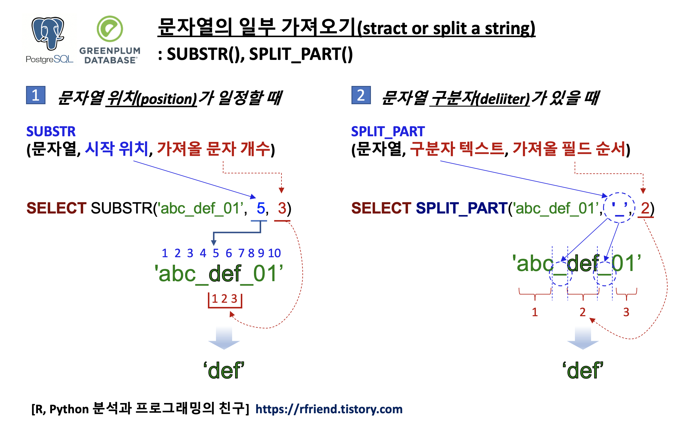
SUBSTR() 함수는 문자열의 포맷이 일정하게 정해져 있어서 위치를 기반으로 문자열의 특정한 일부분만 가져올 때 사용합니다. 반면에, SPLIT_PART() 함수는 문자열에 구분자(delimiter)가 있어서, 이 구분자를 기준으로 문자열을 구분한 후에 특정 순서에 위치한 문자열의 일부분을 가져올 때 사용합니다.
아래에 간단한 예를 들어서 설명하겠습니다.
(1) 위치 기반(position based)으로 문자열의 일부분 가져오기: SUBSTRING(), SUBSTR()
- syntax: SUBSTR(문자열, 시작 위치, 가져올 문자 개수)
substr() 함수와 substring() 함수는 동일합니다.
---------------------------------------------
-- String functions in PostgreSQL
-- substr() vs. split_part()
---------------------------------------------

-- (1) substr(string, from [, count])
-- : Extract substring
-- : when position is fixed

SELECT
	SUBSTR('abc_def_01', 1, 3) AS substr_1
	, SUBSTR('abc_def_01', 5, 3) AS substr_2
	, SUBSTR('abc_def_01', 9, 2) AS substr_3;

--substr_1|substr_2|substr_3|
----------+--------+--------+
--abc     |def     |01      |


-- or equivalently  (same as substring(string from from for count))
SELECT
	SUBSTRING('abc_def_01', 1, 3) AS substr_1
	, SUBSTRING('abc_def_01', 5, 3) AS substr_2
	, SUBSTRING('abc_def_01', 9, 2) AS substr_3;
-- (2) split_part(string text, delimiter text, field int)
-- : Split string on delimiter and return the given field (counting from one)
-- : when deliiter is fixed

SELECT
	SPLIT_PART('abc_def_01', '_', 1) AS split_part_1
	, SPLIT_PART('abc_def_01', '_', 2) AS split_part_2
	, SPLIT_PART('abc_def_01', '_', 3) AS split_part_3;

--split_part_1|split_part_2|split_part_3|
--------------+------------+------------+
--abc         |def         |01          |
이번 포스팅에서는 PostgreSQL, Greenplum 에서 Apahe MADlib 의 함수를 사용하여
(1) 2D array 를 1D array 로 unnest 하기
(Unnest 2D array into 1D array in PostgreSQL using madlib.array_unnest_2d_to_1d() function)
(2) 1D array 에서 순서대로 원소 값을 indexing 하기
하는 방법을 소개하겠습니다.
how to unnest 2D array into 1D array and indexing in PostgreSQL, Greenplum DB
먼저, 예제로 사용할 간단한 2D array를 포함하는 테이블을 만들어 보겠습니다.
--------------------------------------------------------------------------------
-- How to unnest a 2D array into a 1D array in PostgreSQL?
-- [reference] http://madlib.incubator.apache.org/docs/latest/array__ops_8sql__in.html#af057b589f2a2cb1095caa99feaeb3d70
--------------------------------------------------------------------------------

-- Creating a sample 2D array table
DROP TABLE IF EXISTS mat_2d_arr;
CREATE TABLE mat_2d_arr (id int, var_2d int[]);
INSERT INTO mat_2d_arr VALUES
(1,  '{{1, 2, 3}, {4, 5, 6}, {7, 8, 9}}'),
(2,  '{{10, 11, 12}, {13, 14, 15}, {16, 17, 18}}'),
(3,  '{{19, 20, 21}, {22, 23, 24}, {25, 26, 27}}'),
(4,  '{{28, 29, 30}, {31, 32, 33}, {34, 35, 36}}');


SELECT * FROM mat_2d_arr ORDER BY id;

--id|var_2d                            |
----+----------------------------------+
-- 1|{{1,2,3},{4,5,6},{7,8,9}}         |
-- 2|{{10,11,12},{13,14,15},{16,17,18}}|
-- 3|{{19,20,21},{22,23,24},{25,26,27}}|
-- 4|{{28,29,30},{31,32,33},{34,35,36}}|
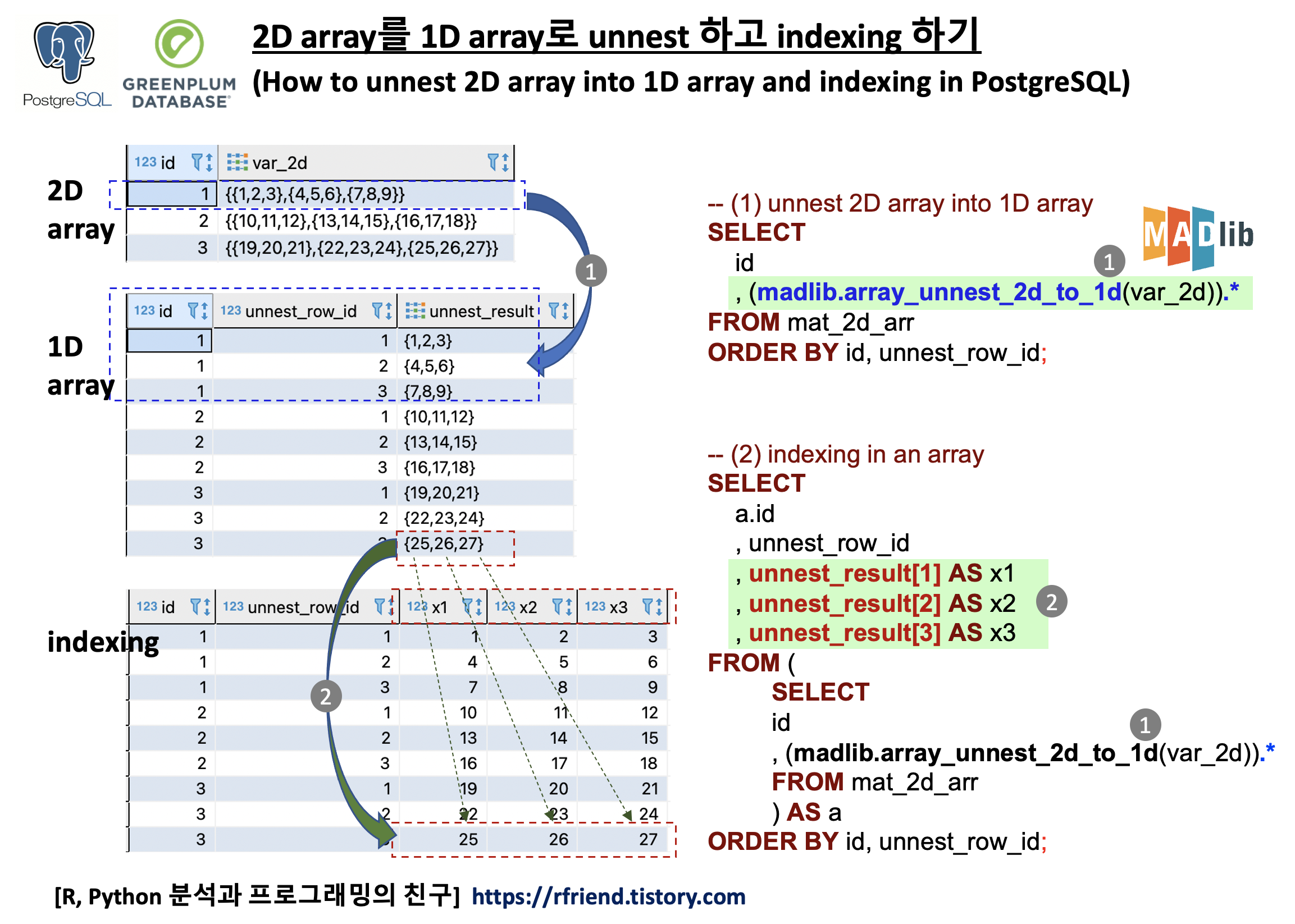
(1) 2D array 를 1D array 로 unnest 하기
(Unnest 2D array into 1D array in PostgreSQL using madlib.array_unnest_2d_to_1d() function)
Apache MADlib 의 madlib.array_unnest_2d_to_1d() 함수를 사용하면 쉽게 PostgreSQL, Greenplum의 2D array를 1D array 로 unnest 할 수 있습니다. madlib.array_unnest_2d_to_1d() 함수는 'unnest_row_id' 와 'unnest_result' 의 2개 칼럼을 반환하므로, 이들 "2개 칼럼 모두"를 반환하라는 의미로 (madlib.array_unnest_2d_to_1d(var_2d)).* 함수의 처음과 끝부분에 괄호 ()로 묶고 마지막에 아스타리스크(.*) 부호를 붙여주었습니다. ().* 를 빼먹지 않도록 주의하세요.
MADlib 함수를 사용하지 않는다면 직접 PL/SQL 사용자 정의 함수나 또는 PL/Python 이나 PL/R 사용자 정의 함수를 정의하고 실행해야 하는데요, 좀 번거롭고 어렵습니다.
-- (1) Unnest 2D array into a 1D array using madlib.array_unnest_2d_to_1d() function
SELECT
	id
	, (madlib.array_unnest_2d_to_1d(var_2d)).*
FROM mat_2d_arr
ORDER BY id, unnest_row_id;

--id|unnest_row_id|unnest_result|
----+-------------+-------------+
-- 1|            1|{1,2,3}      |
-- 1|            2|{4,5,6}      |
-- 1|            3|{7,8,9}      |
-- 2|            1|{10,11,12}   |
-- 2|            2|{13,14,15}   |
-- 2|            3|{16,17,18}   |
-- 3|            1|{19,20,21}   |
-- 3|            2|{22,23,24}   |
-- 3|            3|{25,26,27}   |
-- 4|            1|{28,29,30}   |
-- 4|            2|{31,32,33}   |
-- 4|            3|{34,35,36}   |
아래는 2D array를 1D array로 unnest 하는 사용자 정의함수(UDF) 를 plpgsql 로 정의해서 SQL query 로 호출해서 사용하는 방법입니다.
-- UDF for unnest 2D array into 1D array
CREATE OR REPLACE FUNCTION unnest_2d_1d(ANYARRAY, OUT a ANYARRAY)
  RETURNS SETOF ANYARRAY
  LANGUAGE plpgsql IMMUTABLE STRICT AS
$func$
BEGIN
   FOREACH a SLICE 1 IN ARRAY $1 LOOP
      RETURN NEXT;
   END LOOP;
END
$func$;


-- Unnest 2D array into 1D array using the UDF above
SELECT
	id
	, unnest_2d_1d(var_2d) AS var_1d
FROM mat_2d_arr
ORDER BY 1, 2;

--id|var_1d    |
----+----------+
-- 1|{1,2,3}   |
-- 1|{4,5,6}   |
-- 1|{7,8,9}   |
-- 2|{10,11,12}|
-- 2|{13,14,15}|
-- 2|{16,17,18}|
-- 3|{19,20,21}|
-- 3|{22,23,24}|
-- 3|{25,26,27}|
-- 4|{28,29,30}|
-- 4|{31,32,33}|
-- 4|{34,35,36}|
(2) 1D array 에서 순서대로 원소 값을 indexing 하기
일단 2D array를 1D array 로 unnest 하고 나면, 그 다음에 1D array에서 순서대로 각 원소를 inndexing 해오는 것은 기본 SQL 구문을 사용하면 됩니다. 1D array 안에 각 3개의 원소들이 들어 있으므로, 순서대로 unnest_result[1], unnest_result[2], unnest_result[3] 으로 해서 indexing 을 해오면 아래 예제와 같습니다.
-- (2) Indexing an unnested 1D array
SELECT
	a.id
	, unnest_row_id
	, unnest_result[1] AS x1
	, unnest_result[2] AS x2
	, unnest_result[3] AS x3
FROM (
	SELECT
		id
		, (madlib.array_unnest_2d_to_1d(var_2d)).*
	FROM mat_2d_arr
) AS a
ORDER BY id, unnest_row_id;

--id|unnest_row_id|x1|x2|x3|
----+-------------+--+--+--+
-- 1|            1| 1| 2| 3|
-- 1|            2| 4| 5| 6|
-- 1|            3| 7| 8| 9|
-- 2|            1|10|11|12|
-- 2|            2|13|14|15|
-- 2|            3|16|17|18|
-- 3|            1|19|20|21|
-- 3|            2|22|23|24|
-- 3|            3|25|26|27|
-- 4|            1|28|29|30|
-- 4|            2|31|32|33|
-- 4|            3|34|35|36|
데이터셋에 이상치가 있으면 모델을 훈련시킬 때 적합된 모수에 큰 영향을 줍니다. 따라서 탐색적 데이터 분석을 할 때 이상치(outlier)를 찾고 제거하는 작업이 필요합니다.
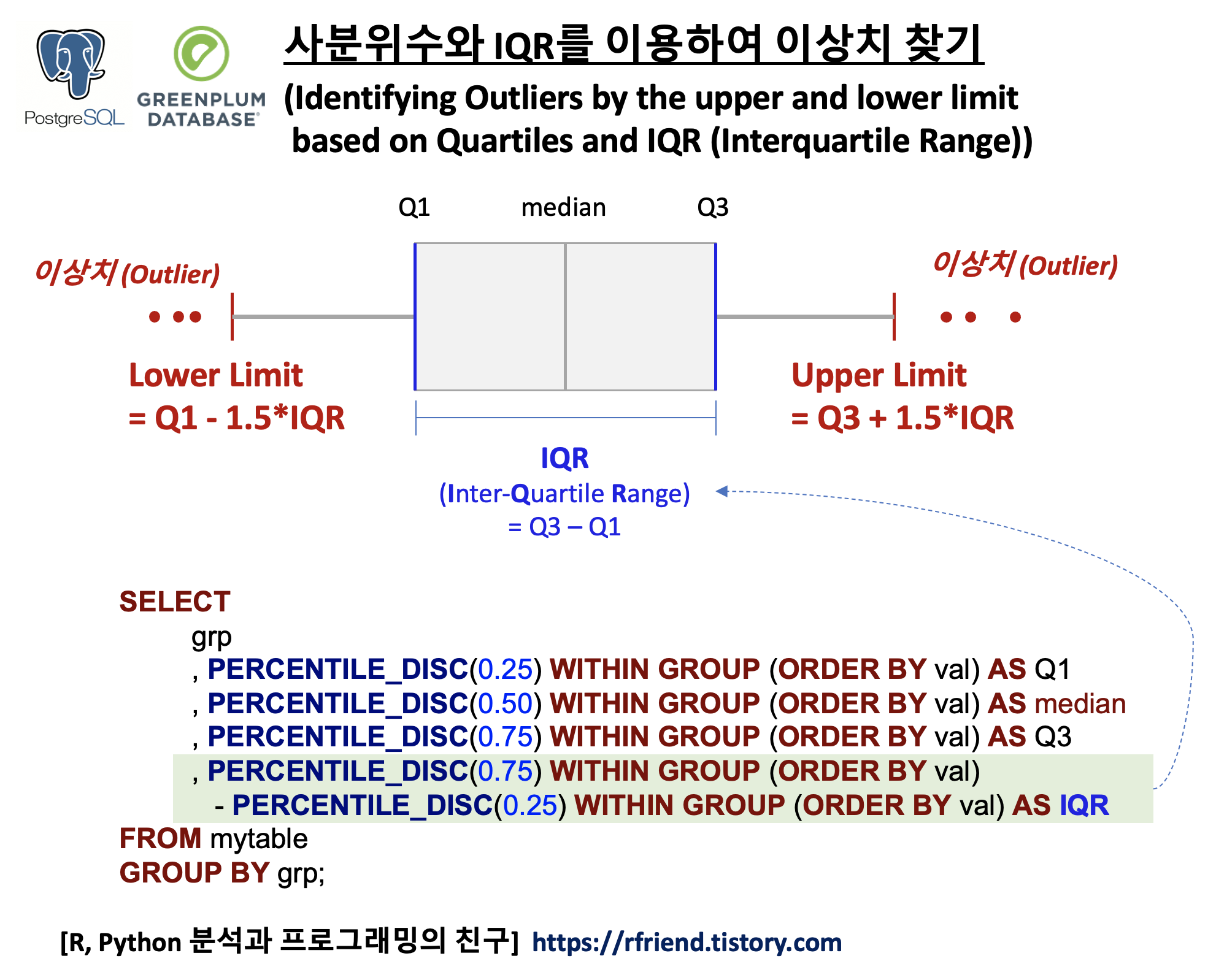
이번 포스팅에서는 PostgreSQL, Greenplum DB에서 SQL의 PERCENTILE_DISC() WITHIN GROUP (ORDER BY) 함수를 사용해서, 사분위수와 IQR 에 기반하여 이상치를 찾고 제거하는 방법(Identifying and removing Outliers by the upper and lower limit based on Quartiles and IQR(Interquartile Range))을 소개하겠습니다.
요약통계량의 평균과 표준편차는 이상치에 매우 민감합니다. 따라서 정규분포가 아니라 이상치가 존재하여 한쪽으로 치우친 분포에서는 (average +-3 * standard deviation) 범위 밖의 값을 이상치로 간주하는 방법은 적합하지 않을 수 있습니다. 반면, 이상치에 덜 민감한 사분위수와 IQR 를 이용하여 이상치를 찾고 제거하는 방법은 간단하게 구현하여 사용할 수 있습니다.
identifying outliers by upper and lower limit based on quartiles and IQR using SQL
먼저, 예제로 사용할 데이터셋 테이블을 만들어보겠습니다. 부산과 서울의 지역(region) 그룹별로 seller_id 별 판매금액(amt) 을 칼럼으로 가지며, 판매금액에 이상치(outliler)를 포함시켰습니다.
PostgreSQL, Greenplum 에서 PERCENTILE_DISC() 함수를 사용하여 사분위수(quartiles)와 IQR(Interquartile Range)를 구할 수 있습니다. 아래 예에서는 지역(region) 별로 1사분위수(Q1), 중앙값(median), 3사분위수(Q3), IQR (Interquartile Range) 를 구해보았습니다.
IQR (Interquartile Range) = Q3 - Q1
-- Quartiles by region groups
-- Interquartile Range (IQR) = Q3-Q1
-- : relatively robust statistic compared to range and std dev for the measure of spread.
SELECT
	region
	, PERCENTILE_DISC(0.25) WITHIN GROUP (ORDER BY amt) AS q1
	, PERCENTILE_DISC(0.50) WITHIN GROUP (ORDER BY amt) AS median
	, PERCENTILE_DISC(0.75) WITHIN GROUP (ORDER BY amt) AS q3
	, PERCENTILE_DISC(0.75) WITHIN GROUP (ORDER BY amt)  -
		PERCENTILE_DISC(0.25) WITHIN GROUP (ORDER BY amt) AS iqr
FROM reg_sales
GROUP BY region
ORDER BY region;

--region|q1 |median|q3 |iqr|
--------+---+------+---+---+
--Busan |350|   390|450|100|
--Seoul |350|   380|440| 90|
사분위수와 IQR 를 이용하여 이상치를 찾는 방식(identifying outliers by upper and lower limit based on quartiles and IQR using SQL in PostgreSQL)은 아래와 같습니다. (포스팅 상단의 도식 참조)
* Upper Limit = Q1 - 1.5 * IQR
* Lower Limit = Q3 + 1.5 * IQR
if value > Upper Limit then 'Outlier'
or if value < Lower Limit then 'Outlier'
-- Identifying outliers by the upper and lower limit based on Quartiles and IQR as:
-- : Lower Limit = Q1 – 1.5 * IQR
-- : Upper Limit = Q3 + 1.5 * IQR

WITH stats AS (
	SELECT
	region
	, PERCENTILE_DISC(0.25) WITHIN GROUP (ORDER BY amt) AS q1
	, PERCENTILE_DISC(0.75) WITHIN GROUP (ORDER BY amt) AS q3
	, PERCENTILE_DISC(0.75) WITHIN GROUP (ORDER BY amt)  -
		PERCENTILE_DISC(0.25) WITHIN GROUP (ORDER BY amt) AS iqr
	FROM reg_sales
	GROUP BY region
)
SELECT
	r.*
FROM reg_sales AS r
LEFT JOIN stats AS s ON r.region = s.region
WHERE r.amt < (s.q1 - 1.5 * s.iqr) OR r.amt > (s.q3 + 1.5 * s.iqr) -- identifying outliers
ORDER BY region, amt;

--region|seller_id|amt |
--------+---------+----+
--Busan |        1|  10|
--Busan |        9|3200|
--Busan |       10|4600|
--Seoul |        1|  20|
--Seoul |       10|2500|
아래의 예에서는 사분위수와 IQR에 기반하여 이상치를 제거 (Removing outliers by upper and lower limit based on quartiles and IQR using SQL in PostgreSQL) 하여 보겠습니다.
-- Removing outliers by the upper and lower limit based on Quartiles and IQR as:
-- : Lower Limit = Q1 – 1.5 * IQR
-- : Upper Limit = Q3 + 1.5 * IQR

WITH stats AS (
	SELECT
	region
	, PERCENTILE_DISC(0.25) WITHIN GROUP (ORDER BY amt) AS q1
	, PERCENTILE_DISC(0.75) WITHIN GROUP (ORDER BY amt) AS q3
	, PERCENTILE_DISC(0.75) WITHIN GROUP (ORDER BY amt)  -
		PERCENTILE_DISC(0.25) WITHIN GROUP (ORDER BY amt) AS iqr
	FROM reg_sales
	GROUP BY region
)
SELECT
	r.*
FROM reg_sales AS r
LEFT JOIN stats AS s ON r.region = s.region
WHERE r.amt > (s.q1 - 1.5 * s.iqr) AND r.amt < (s.q3 + 1.5 * s.iqr) -- removing outliers
ORDER BY region, amt;

--region|seller_id|amt|
--------+---------+---+
--Busan |        2|310|
--Busan |        3|350|
--Busan |        4|380|
--Busan |        5|390|
--Busan |        6|430|
--Busan |        7|450|
--Busan |        8|450|
--Seoul |        2|300|
--Seoul |        3|350|
--Seoul |        4|370|
--Seoul |        5|380|
--Seoul |        6|400|
--Seoul |        7|410|
--Seoul |        8|440|
--Seoul |        9|460|
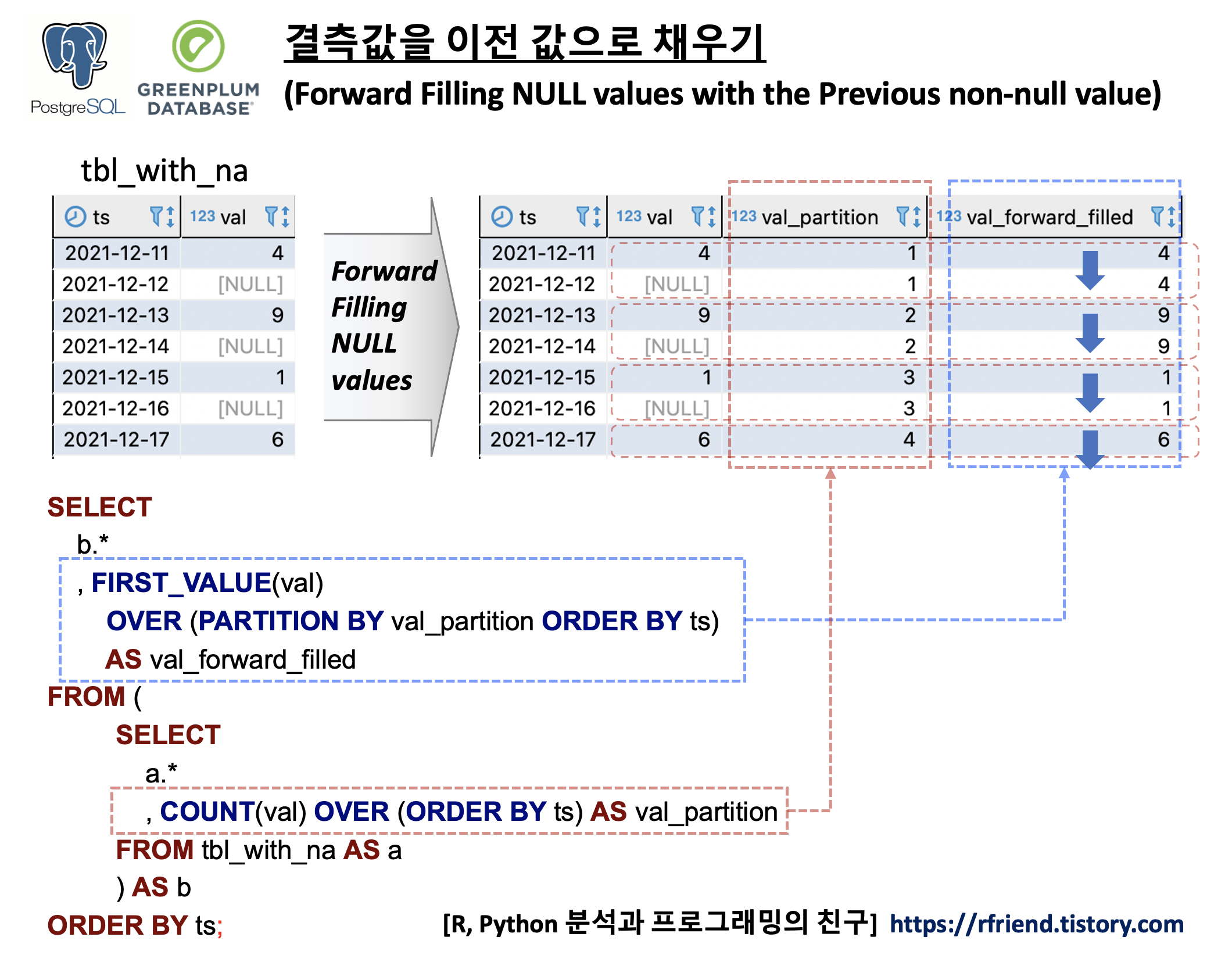
데이터 분석을 하다보면 데이터 전처리 단계에서 '결측값 확인 및 처리(handling missing values) '가 필요합니다.
시계열 데이터의 결측값을 처리하는 방법에는 보간(interpolation), 이전/이후 값으로 대체, 이동평균(moving average)으로 대체 등 여러가지 방법(https://rfriend.tistory.com/682)이 있습니다.
이번 포스팅에서는 가장 간단한 방법으로서 PostgreSQL, Greenplum DB에서 SQL로 first_value() window function을 사용해서 할 수 있는 '결측값을 이전 값으로 채우기' 또는 '결측값을 이후 값으로 채이기' 하는 방법을 소개하겠습니다.
(1) 결측값을 이전 값으로 채우기
(Forward filling NULL values with the previous non-null value)
(2) 여러개 칼럼의 결측값을 이전 값으로 채우기
(Forward filling NULL values in Multiple Columns with the previous non-null value)
(3) 그룹별로 결측값을 이전 값으로 채우기
(Forward filling NULL values by Group with the previous non-null value)
(4) 결측값을 이후 값으로 채우기
(Backward filling NULL values with the next non-null value)
PostgreSQL, Greenplum, forward filling NULL values with the previous non-null value
결측값을 시계열데이터의 TimeStamp 를 기준으로 정렬한 상태에서 SQL로 결측값을 이전의 실측값으로 채우는 방법의 핵심은 FIRST_VALUE() Window Function 을 사용하는 것입니다. FIRST_VALUE() 의 구문은 아래와 같으며, OVER(PARTITION BY column_name ORDER BY TimeStamp_column_name) 의 기능은 위의 예제에 대한 도식의 빨강, 파랑 박스와 화살표를 참고하시기 바랍니다.
-- PostgreSQL FIRST_VALUE() Window Function syntax

FIRST_VALUE ( expression )
OVER (
    [PARTITION BY partition_expression, ... ]
    ORDER BY sort_expression [ASC | DESC], ...
)
(1) 결측값을 이전 값으로 채우기
(Forward filling NULL values with the previous non-null value)
먼저, 날짜를 나타내는 'ts' 칼럼과 결측값을 가지는 'val' 칼럼으로 구성된 예제 테이블을 만들어보겠습니다.
-- creating a sample dataset with NULL values
DROP TABLE IF EXISTS tbl_with_na;
CREATE TABLE tbl_with_na (
	ts DATE NOT NULL
	, val int
);

INSERT INTO tbl_with_na VALUES
('2021-12-11', 4)
, ('2021-12-12',NULL)
, ('2021-12-13', 9)
, ('2021-12-14', NULL)
, ('2021-12-15', 1)
, ('2021-12-16', NULL)
, ('2021-12-17', 6)
;

SELECT * FROM tbl_with_na ORDER BY ts;

--ts        |val|
------------+---+
--2021-12-11|  4|
--2021-12-12|   |
--2021-12-13|  9|
--2021-12-14|   |
--2021-12-15|  1|
--2021-12-16|   |
--2021-12-17|  6|
이제 FIRST_VALUE() OVER(), COUNT() OVER() 의 window function 을 사용해서 결측값을 이전 실측값으로 채워보겠습니다.
-----------------------------------------------------
-- (1) Forward Filling NULL values
-----------------------------------------------------
SELECT
	b.*
	, FIRST_VALUE(val)
		OVER (PARTITION BY val_partition ORDER BY ts)
			AS val_forward_filled
FROM (
	SELECT
		a.*
		, count(val) OVER (ORDER BY ts) AS val_partition
	FROM tbl_with_na AS a
	) AS b
ORDER BY ts;

--ts        |val|val_partition|val_forward_filled|
------------+---+-------------+------------------+
--2021-12-11|  4|            1|                 4|
--2021-12-12|   |            1|                 4|
--2021-12-13|  9|            2|                 9|
--2021-12-14|   |            2|                 9|
--2021-12-15|  1|            3|                 1|
--2021-12-16|   |            3|                 1|
--2021-12-17|  6|            4|                 6|
(2) 여러개 칼럼의 결측값을 이전 값으로 채우기
(Forward filling NULL values in Multiple Columns with the previous non-null value)
먼저, 날짜를 나타내는 칼럼 'ts'와 측정값을 가지는 2개의 칼럼 'val_1', 'val_2'로 구성된 예제 테이블을 만들어 보겠습니다.
-- creating a sample table with NULL values in multiple columns
DROP TABLE IF EXISTS tbl_with_na_mult_cols;
CREATE TABLE tbl_with_na_mult_cols (
	ts DATE NOT NULL
	, val_1 int
	, val_2 int
);

INSERT INTO tbl_with_na_mult_cols VALUES
('2021-12-11', 1, 5)
, ('2021-12-12',NULL, NULL)
, ('2021-12-13', 2, 6)
, ('2021-12-14', NULL, 7)
, ('2021-12-15', 3, NULL)
, ('2021-12-16', NULL, NULL)
, ('2021-12-17', 4, 8)
;

SELECT * FROM tbl_with_na_mult_cols ORDER BY ts;

--ts        |val_1|val_2|
------------+-----+-----+
--2021-12-11|    1|    5|
--2021-12-12|     |     |
--2021-12-13|    2|    6|
--2021-12-14|     |    7|
--2021-12-15|    3|     |
--2021-12-16|     |     |
--2021-12-17|    4|    8|
다음으로 결측값을 채우려는 여러개의 각 칼럼마다 FIRST_VALUE() OVER(), COUNT() OVER() 의 window function 을 사용해서 결측값을 이전 값으로 채워보겠습니다.
------------------------------------------------------------------
-- (2) Forward Filling NULL values in Multiple Columns
------------------------------------------------------------------
SELECT
	b.ts
	, b.val_1
	, b.val_1_partition
	, FIRST_VALUE(val_1)
		OVER (PARTITION BY val_1_partition ORDER BY ts)
		AS val_1_fw_filled
	, b.val_2
	, b.val_2_partition
	, FIRST_VALUE(val_2)
		OVER (PARTITION BY val_2_partition ORDER BY ts)
		AS val_2_fw_filled
FROM (
	SELECT
		a.*
		, count(val_1) OVER (ORDER BY ts) AS val_1_partition
		, count(val_2) OVER (ORDER BY ts) AS val_2_partition
	FROM tbl_with_na_mult_cols AS a
	) AS b
ORDER BY ts;

--ts        |val_1|val_1_partition|val_1_fw_filled|val_2|val_2_partition|val_2_fw_filled|
------------+-----+---------------+---------------+-----+---------------+---------------+
--2021-12-11|    1|              1|              1|    5|              1|              5|
--2021-12-12|     |              1|              1|     |              1|              5|
--2021-12-13|    2|              2|              2|    6|              2|              6|
--2021-12-14|     |              2|              2|    7|              3|              7|
--2021-12-15|    3|              3|              3|     |              3|              7|
--2021-12-16|     |              3|              3|     |              3|              7|
--2021-12-17|    4|              4|              4|    8|              4|              8|
(3) 그룹별로 결측값을 이전 값으로 채우기
(Forward filling NULL values by Group with the previous non-null value)
이번에는 2개의 그룹('a', 'b')이 있고, 'val' 칼럼에 결측값이 있는 예제 데이터 테이블을 만들어보겠습니다.
-- creating a sample dataset with groups
DROP TABLE IF EXISTS tbl_with_na_grp;
CREATE TABLE tbl_with_na_grp (
	ts DATE NOT NULL
	, grp TEXT NOT NULL
	, val int
);

INSERT INTO tbl_with_na_grp VALUES
('2021-12-11', 'a',1) -- GROUP 'a'
, ('2021-12-12','a', NULL)
, ('2021-12-13', 'a', 2)
, ('2021-12-14', 'a', NULL)
, ('2021-12-15', 'a', 3)
, ('2021-12-16', 'a', NULL)
, ('2021-12-17', 'a', 4)
, ('2021-12-11', 'b', 11) -- GROUP 'b'
, ('2021-12-12', 'b', NULL)
, ('2021-12-13', 'b', 13)
, ('2021-12-14', 'b', NULL)
, ('2021-12-15', 'b', 15)
, ('2021-12-16', 'b', NULL)
, ('2021-12-17', 'b', 17)
;

SELECT * FROM tbl_with_na_grp ORDER BY grp, ts;

--ts        |grp|val|
------------+---+---+
--2021-12-11|a  |  1|
--2021-12-12|a  |   |
--2021-12-13|a  |  2|
--2021-12-14|a  |   |
--2021-12-15|a  |  3|
--2021-12-16|a  |   |
--2021-12-17|a  |  4|
--2021-12-11|b  | 11|
--2021-12-12|b  |   |
--2021-12-13|b  | 13|
--2021-12-14|b  |   |
--2021-12-15|b  | 15|
--2021-12-16|b  |   |
--2021-12-17|b  | 17|
이제 그룹 별로(OVER (PARTITION BY grp, val_partition ORDER BY ts)) 이전 값으로 채우기(FIRST_VALUE(val))를 해보겠습니다.
----------------------------------------------------------
-- (3) Forward Filling NULL values by Group
----------------------------------------------------------
SELECT
	b.*
	, FIRST_VALUE(val)
		OVER (PARTITION BY grp, val_partition ORDER BY ts)
		AS val_filled
FROM (
	SELECT
		a.*
		, count(val)
			OVER (PARTITION BY grp ORDER BY ts)
			AS val_partition
	FROM tbl_with_na_grp AS a
	) AS b
ORDER BY grp, ts;

--ts        |grp|val|val_partition|val_filled|
------------+---+---+-------------+----------+
--2021-12-11|a  |  1|            1|         1|
--2021-12-12|a  |   |            1|         1|
--2021-12-13|a  |  2|            2|         2|
--2021-12-14|a  |   |            2|         2|
--2021-12-15|a  |  3|            3|         3|
--2021-12-16|a  |   |            3|         3|
--2021-12-17|a  |  4|            4|         4|
--2021-12-11|b  | 11|            1|        11|
--2021-12-12|b  |   |            1|        11|
--2021-12-13|b  | 13|            2|        13|
--2021-12-14|b  |   |            2|        13|
--2021-12-15|b  | 15|            3|        15|
--2021-12-16|b  |   |            3|        15|
--2021-12-17|b  | 17|            4|        17|
(4) 결측값을 이후 값으로 채우기
(Backward filling NULL values with the next non-null value)
결측값을 이전 값(previous non-null value)이 아니라 이후 값(next non-null value) 으로 채우려면 (1)번의 SQL 코드에서 OVER (ORDER BY ts DESC)) 처럼 내림차순으로 정렬(sorting in DESCENDING order) 해준 후에 FIRST_VALUE() 를 사용하면 됩니다.
-----------------------------------------------------
-- (4) Backward Filling NULL values
-----------------------------------------------------

SELECT
	b.*
	, FIRST_VALUE(val)
		OVER (PARTITION BY grp, val_partition ORDER BY ts DESC)
		AS val_filled
FROM (
	SELECT
		a.*
		, count(val)
			OVER (PARTITION BY grp ORDER BY ts DESC)
			AS val_partition
	FROM tbl_with_na_grp AS a
	) AS b
ORDER BY grp, ts;

--ts        |grp|val|val_partition|val_filled|
------------+---+---+-------------+----------+
--2021-12-11|a  |  1|            4|         1|
--2021-12-12|a  |   |            3|         2|
--2021-12-13|a  |  2|            3|         2|
--2021-12-14|a  |   |            2|         3|
--2021-12-15|a  |  3|            2|         3|
--2021-12-16|a  |   |            1|         4|
--2021-12-17|a  |  4|            1|         4|
--2021-12-11|b  | 11|            4|        11|
--2021-12-12|b  |   |            3|        13|
--2021-12-13|b  | 13|            3|        13|
--2021-12-14|b  |   |            2|        15|
--2021-12-15|b  | 15|            2|        15|
--2021-12-16|b  |   |            1|        17|
--2021-12-17|b  | 17|            1|        17|
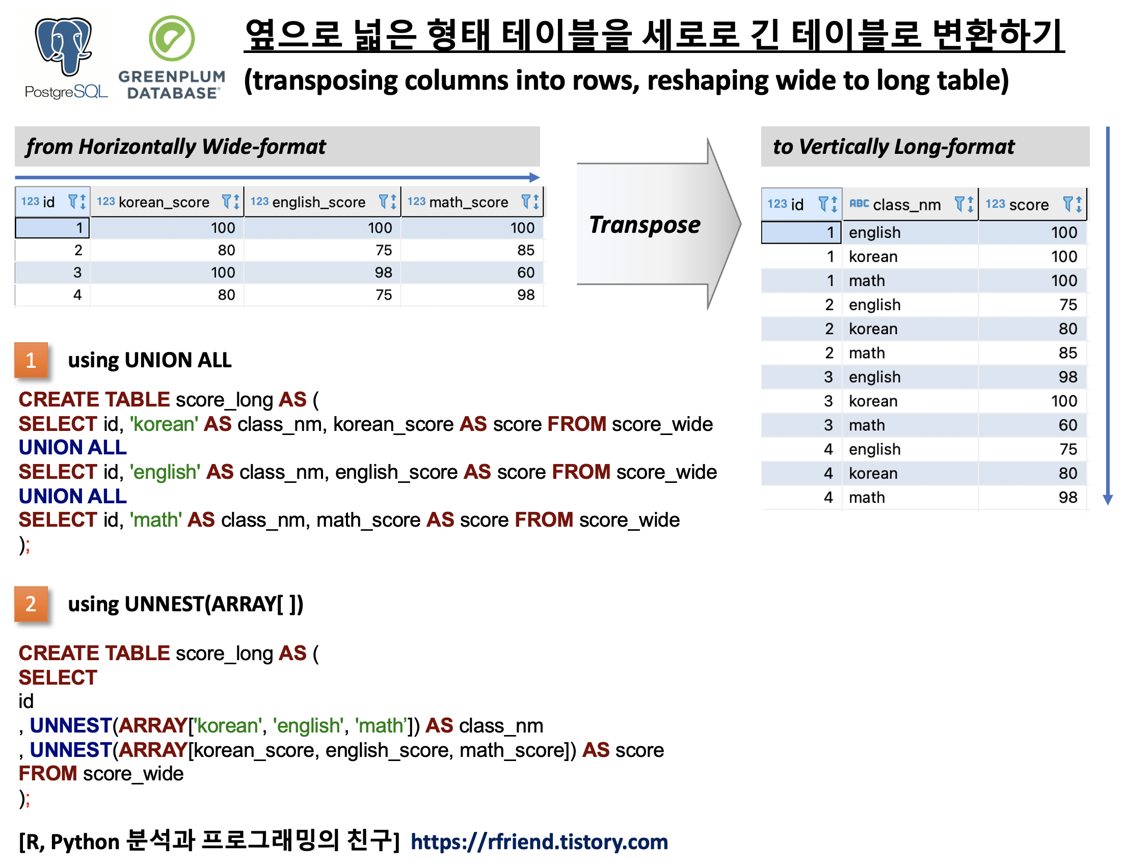
지난번 포스팅에서는 PostgreSQL, Greenplum DB에서 옆으로 넓은 테이블(horizontally wide-format table)을 세로로 긴 테이블(vertically long-format table)로 변환(transpose)하는 2가지 방법을 소개하였습니다. (https://rfriend.tistory.com/713)
이번 포스팅에서는 반대로, PostgreSQL, Greenplum DB에서 세로로 긴 테이블을 가로로 넓은 테이블로 Pivot 하는 방법(Pivoting table, converting long-format table to wide-format table)을 소개하겠습니다. 보통 탐색적 데이터 분석, 통계 분석, 기계학습 등의 분석을 할 때는 pivot table 한 후의 각 ID별로 여러개의 칼럼이 옆으로 넓게 붙은 형태의 테이블을 사용합니다.
* PostgreSQL과 Greenplum 에서 각각 다른 함수를 사용하는 것에 유의하세요.
(1) PostgreSQL에서 tablefunc extension의 crosstab() 함수를 이용해 테이블 피봇하기
(Pivoting table using crosstab() function in PostgreSQL)
(2) Greenplum 에서 Apache MADlib의 pivot() 함수를 이용해 테이블 피봇하기
(Pivoting table using Apache MADlib's pivot() function in Greenplum)
(3) Manual 하게 Select 후 Join 해서 테이블 피봇하기
(Pivoting table by select and join manually)
PostgreSQL, Greenplum, pivoting table, reshaping from long-format to wide-format
먼저, 예제로 사용할 간단한 예제 테이블을 만들어보겠습니다. 학생 ID별로 과목(class_nm) 별 점수(score) 를 저장해놓은 테이블입니다.
--------------------------------------------------------------------------------
-- Pivoting table using crosstab() function in PostgreSql 9.4+
-- [ref] https://www.postgresql.org/docs/9.4/tablefunc.html
-- [ref] https://learnsql.com/blog/creating-pivot-tables-in-postgresql-using-the-crosstab-function/
--------------------------------------------------------------------------------

DROP TABLE IF EXISTS score_long;
CREATE TABLE score_long (
	id int NOT null
	, class_nm TEXT
	, score int
);

INSERT INTO score_long VALUES
 (1,'english' , 100)
, (1,'korean' , 100)
, (1,'math', 100)
, (2,'english', 75)
, (2,'korean', 80)
, (2,'math', 85)
, (3,'english', 98)
, (3,'korean' , 100)
, (3,'math', 60)
, (4,'english', 75)
, (4,'korean', 80)
, (4,'math', 98)
;

SELECT * FROM score_long ORDER BY id, class_nm;
--id|class_nm|score
----+--------+-----+
-- 1|english |  100|
-- 1|korean  |  100|
-- 1|math    |  100|
-- 2|english |   75|
-- 2|korean  |   80|
-- 2|math    |   85|
-- 3|english |   98|
-- 3|korean  |  100|
-- 3|math    |   60|
-- 4|english |   75|
-- 4|korean  |   80|
-- 4|math    |   98|
(1) PostgreSQL에서 tablefunc extension의 crosstab() 함수를 이용해 테이블 피봇하기
(Pivoting table using crosstab() function in PostgreSQL)
세로로 긴 테이블을 가로로 넓은 테이블로 pivot 할 때 사용되는 crosstab() 함수는 PostgreSQL 버전 8.3 이 배포되었을 때 처음 소개되었던 tablefunc extension 에 포함되었습니다. 따라서 tablefunc extension 을 처음 사용하는 경우라면
CREATE EXTENSION tablefunc; 로 활성화시켜준 후에 crosstab() 함수를 호출해서 사용할 수 있습니다.
crosstab() 함수는 SELECT 문의 FROM 절에 사용이 되므로 처음 사용하는 분이라면 좀 낯설게 여길 수도 있겠습니다. crosstab() 함수에서 SELECT 문은 3개의 칼럼을 반환합니다.
(칼럼 1) 첫번째 칼럼은 각 관측치를 구분하는 ID (identifier) 칼럼입니다. 위의 예에서는 학생들의 ID가 이에 해당합니다.
(칼럼 2) 두번째 칼럼은 pivot table 에서의 범주(categories)에 해당하는 칼럼입니다. pivot을 하게 되면 각 칼럼으로 변환이 됩니다. 위의 예에서는 과목명(class_nm) 칼럼이 이에 해당합니다.
(칼럼 3) 세번째 칼럼은 pivot table 의 각 셀에 할당이 될 값(value)에 해당하는 칼럼입니다. 위의 예에서는 점수(score) 칼럼이 이에 해당합니다.
crosstab() 함수안에 SQL query로 위의 3개 칼럼을 select 한 결과를, AS final_result() 에서 pivot table 에서 재표현할 칼럼 이름과 데이터 유형을 정의해주면 됩니다.
-- (1) Pivoting table using PostgreSQL's crosstab() function
-- Enabling the Crosstab Function
-- : The crosstab() function is part of a PostgreSQL extension called tablefunc.
CREATE EXTENSION tablefunc;

-- Pivoting table
--: The crosstab() function receives an SQL SELECT command as a parameter.
SELECT *
FROM
	crosstab(
		'select id, class_nm, score
		from score_long
		order by 1, 2')
	AS final_result(id int, english_score int, korean_score int, math_score int);

--id|english_score|korean_score|math_score|
----+-------------+------------+----------+
-- 1|          100|         100|       100|
-- 2|           75|          80|        85|
-- 3|           98|         100|        60|
-- 4|           75|          80|        98|
(2) Greenplum 에서 Apache MADlib의 pivot() 함수를 이용해 테이블 피봇하기
(Pivoting table using Apache MADlib's pivot() function in Greenplum)
Greenplum 에서는 PostgreSQL에서 사용했던 crosstab() 함수를 사용할 수 없습니다 대신 Greenplum 에서는 테이블을 pivot 하려고 할 때 Apache MADlib의 pivot() 함수를 사용합니다. 아래의 madlib.pivot() 함수 안의 구문(syntax)을 참고해서 각 매개변수 항목에 순서대로 입력을 해주면 됩니다.
--------------------------------------------------------------------------------
-- Pivoting table using crosstab() function in Greenplum
-- [ref] https://madlib.apache.org/docs/latest/group__grp__pivot.html
--------------------------------------------------------------------------------

-- Pivoting table using Apache MADlib's pivot() function

DROP TABLE IF EXISTS score_pivot;
SELECT madlib.pivot(
	'score_long' 		-- source_table,
	, 'score_pivot' 	-- output_table,
	, 'id' 					-- index,
	, 'class_nm' 		-- pivot_cols,
	, 'score' 			-- pivot_values,
	, 'avg' 				-- aggregate_func,
	, 'NULL'			-- fill_value,
	, 'False'			-- keep_null,
);


SELECT * FROM score_pivot ORDER BY id;
--id|score_avg_class_nm_english|score_avg_class_nm_korean|score_avg_class_nm_math|
--+--------------------------+-------------------------+-----------------------+
-- 1|      100.0000000000000000|     100.0000000000000000|   100.0000000000000000|
-- 2|       75.0000000000000000|      80.0000000000000000|    85.0000000000000000|
-- 3|       98.0000000000000000|     100.0000000000000000|    60.0000000000000000|
-- 4|       75.0000000000000000|      80.0000000000000000|    98.0000000000000000|
칼럼 이름이 자동으로 설정('피봇값_집계함수_카테고리 칼럼이름' 형식)이 되는데요, 만약 칼럼 이름을 사용자의 입맛에 맞게 새로 바꿔주고 싶으면 ALTER TABLE table_name RENAME COLUMN old_column TO new_column; 을 사용해서 바꿔주세요.
-- Renaming the column names
ALTER TABLE score_pivot
RENAME COLUMN score_avg_class_nm_english TO english_score;

ALTER TABLE score_pivot
RENAME COLUMN score_avg_class_nm_korean TO korean_score;

ALTER TABLE score_pivot
RENAME COLUMN score_avg_class_nm_math TO math_score;


SELECT * FROM score_pivot ORDER BY id;
--id|english_score       |korean_score        |math_score          |
----+--------------------+--------------------+--------------------+
-- 1|100.0000000000000000|100.0000000000000000|100.0000000000000000|
-- 2| 75.0000000000000000| 80.0000000000000000| 85.0000000000000000|
-- 3| 98.0000000000000000|100.0000000000000000| 60.0000000000000000|
-- 4| 75.0000000000000000| 80.0000000000000000| 98.0000000000000000|
(3) Manual 하게 Select 후 Join 해서 테이블 피봇하기
(Pivoting table by select and join manually)
물론, 피봇한 후의 테이블에서 칼럼 개수가 몇 개 안된다면 수작업으로 조건절로 SELECT 하여 JOIN 을 해서 새로운 테이블을 만들어 주는 방법도 가능합니다. 다만, pivot table 의 칼럼 개수가 수십, 수백개 된다면 이처럼 수작업으로 일일이 하나씩 SELECT 한 후에 JOIN 을 하는게 매우 번거롭고, 시간이 오래걸리고, 자칫 human error 를 만들 수도 있으니 위의 함수를 사용하는 것이 보다 나아보입니다.
-- (3) Piovting table using join manually
WITH english AS (
	SELECT id, score AS english_score
	FROM score_long
	WHERE class_nm = 'english'
), korean AS (
	SELECT id, score AS korean_score
	FROM score_long
	WHERE class_nm = 'korean'
), math AS (
	SELECT id, score AS math_score
	FROM score_long
	WHERE class_nm = 'math'
)
SELECT * FROM english
LEFT JOIN korean USING(id)
LEFT JOIN math USING(id);

--id|english_score|korean_score|math_score|
----+-------------+------------+----------+
-- 1|          100|         100|       100|
-- 2|           75|          80|        85|
-- 3|           98|         100|        60|
-- 4|           75|          80|        98|
탐색적 데이터분석, 통계나 기계학습 모델링을 할 때의 데이터 형태를 보면 관측치의 식별자 ID(identifier) 별로 하나의 행(row)에 여러개의 특성정보(features)를 여러개의 칼럼(columns)으로 해서 옆으로 넓게 (horizontally wide format) 만든 데이터셋을 사용합니다.
그런데 Database의 Table 은 이와는 다르게, 보통 식별자 ID 별로 칼럼 이름(column name)과 측정값(measured value)을 여러개의 행(rows)으로 해서 세로로 길게 (vertically long format) 만든 테이블로 데이터를 관리합니다. Vertically Long Format 의 테이블이 새로 생성되는 데이터를 추가(insert into)하거나 삭제(delete from) 하기도 쉽고, 그룹별로 연산 (group by operation) 을 하기에도 쉽습니다. 그리고 API 서비스와 DB를 연계할 때도 세로로 긴 형태의 테이블이 사용됩니다.
(통계/기계학습을 하려고 할때는 DB로 부터 Query를 해서 Cross-tab 을 하여 horizontally wide format 의 DataFrame이나 Array 로 바꾸어서 이후 분석을 진행합니다.)
그럼, PostgreSQL, Greenplum DB에서 옆으로 넓은 형태의 테이블을 세로로 긴 형태의 테이블로 변형하는 2가지 방법을 소개하겠습니다. (Transposing columns into rows in PostgreSQL, Greenplum) (Reshaping horizontally wide-format into verticaly long-format table in PostgreSQL, Greenplum)
(1) UNION ALL 함수를 이용하여 여러개의 칼럼을 행으로 변환하기
(2) UNNEST() 함수를 이용하여 여러개의 칼럼을 행으로 변환하기
PostgreSQL, Greenplum, Transposing columns into rows, Reshaping wide to long format table
먼저, 예제로 사용한 간단한 테이블을 생성해 보겠습니다. 학생 ID 별로 국어, 영어, 수학, 과학, 역사, 체육 점수를 옆으로 넓은 형태(horizontally wide-format)로 저장해놓은 테이블입니다.
----------------------------------------------
-- Transposing columns into rows
-- (1) UNION ALL
-- (2) UNNEST()
----------------------------------------------

-- creating a sample table
DROP TABLE IF EXISTS score_wide;
CREATE TABLE score_wide (
	id int NOT NULL
	, korean_score int
	, english_score int
	, math_score int
	, physics_score int
	, history_score int
	, athletics_score int
);

INSERT INTO score_wide VALUES
(1, 100, 100, 100, 100, 100, 90)
, (2, 80, 75, 85, 80, 60, 100)
, (3, 100, 98, 60, 55, 95, 85)
, (4, 80, 75, 98, 100, 85, 95);


SELECT * FROM score_wide ORDER BY id;

--id|korean_score|english_score|math_score|physics_score|history_score|athletics_score|
----+------------+-------------+----------+-------------+-------------+---------------+
-- 1|         100|          100|       100|          100|          100|             90|
-- 2|          80|           75|        85|           80|           60|            100|
-- 3|         100|           98|        60|           55|           95|             85|
-- 4|          80|           75|        98|          100|           85|             95|
(1) UNION ALL 함수를 이용하여 여러개의 칼럼을 행으로 변환하기
일반적으로 많이 알려져 있고, 또 실행 성능도 다음에 소개할 UNNEST() 보다 상대적으로 조금 더 좋습니다.
하지만 아래의 예제 코드를 보면 알 수 있는 것처럼, 칼럼의 개수가 여러개일 경우 코드가 길어지고 동일한 코드 항목 항목이 반복되어서 복잡해보이는 단점이 있습니다.
-- (1) using UNION ALL
DROP TABLE IF EXISTS score_long_union;
CREATE TABLE score_long_union AS (
	SELECT id, 'korean' AS class_nm, korean_score AS score FROM score_wide
	UNION ALL
	SELECT id, 'english' AS class_nm, english_score AS score FROM score_wide
	UNION ALL
	SELECT id, 'math' AS class_nm, math_score AS score FROM score_wide
	UNION ALL
	SELECT id, 'physics' AS class_nm, physics_score AS score FROM score_wide
	UNION ALL
	SELECT id, 'history' AS class_nm, history_score AS score FROM score_wide
	UNION ALL
	SELECT id, 'athletics' AS class_nm, athletics_score AS score FROM score_wide
);


SELECT * FROM score_long_union ORDER BY id, class_nm;

--id|class_nm |score|
----+---------+-----+
-- 1|athletics|   90|
-- 1|english  |  100|
-- 1|history  |  100|
-- 1|korean   |  100|
-- 1|math     |  100|
-- 1|physics  |  100|
-- 2|athletics|  100|
-- 2|english  |   75|
-- 2|history  |   60|
-- 2|korean   |   80|
-- 2|math     |   85|
-- 2|physics  |   80|
-- 3|athletics|   85|
-- 3|english  |   98|
-- 3|history  |   95|
-- 3|korean   |  100|
-- 3|math     |   60|
-- 3|physics  |   55|
-- 4|athletics|   95|
-- 4|english  |   75|
-- 4|history  |   85|
-- 4|korean   |   80|
-- 4|math     |   98|
-- 4|physics  |  100|
(2) UNNEST() 함수를 이용하여 여러개의 칼럼을 행으로 변환하기
다음으로, UNNEST() 함수를 사용하는 방법은 위의 UNION ALL 대비 코드가 한결 간결해서 가독성이 좋습니다.
반면에, UNNEST() 함수를 사용하면 연산이 된 후의 ARRAY 에 대해서는 INDEX가 지원이 안되다보니 위의 UNION ALL 대비 상대적으로 실행 성능이 떨어지는 단점이 있습니다.(UNION ALL 방법이 UNNEST() 방법보다 약 2배 정도 성능이 빠름.)