[Python] scipy를 이용한 시계열 데이터 보간 (interpolation of time series data using scipy)
Python 분석과 프로그래밍/Python 통계분석 2021. 9. 7. 00:17시계열 데이터를 분석할 때 꼭 확인하고 처리해야 하게 있는데요, 바로 결측값 여부 확인과 결측값 처리입니다.
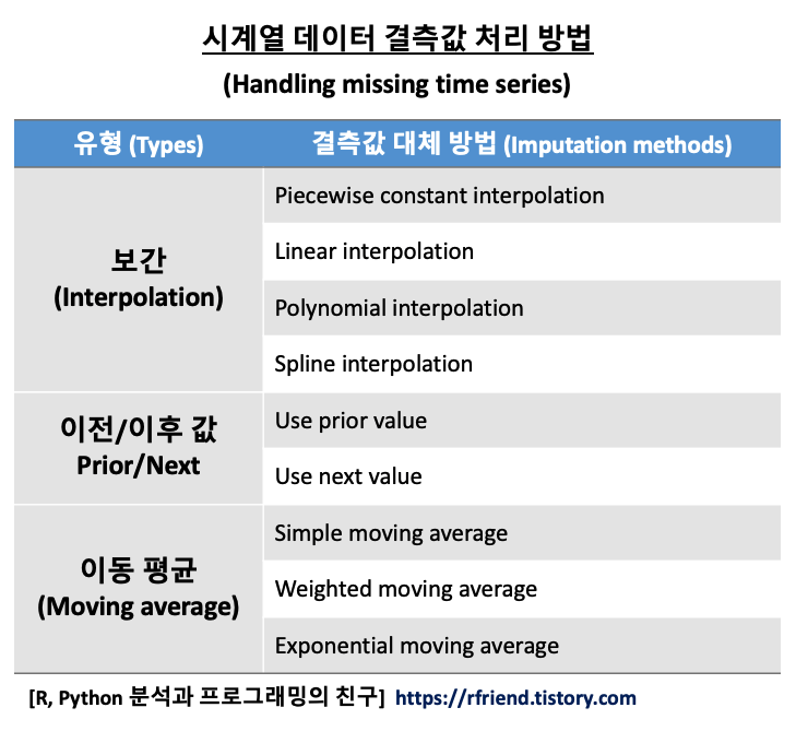
시계열 데이터의 결측값을 처리하는 방법에는
(1) 보간 (Interpolation)
(2) 이전 값 또는 다음 값 이용 (previous/next value)
(3) 이동 평균 (Moving average)
등의 여러가지 방법이 있습니다.
[ 시계열 데이터 결측값 처리 방법 (How to handle the time series missing data) ]
아래의 보간(Interpolation)에 대한 내용은 Wikipedia 의 내용을 번역하여 소개합니다.
데이터 분석의 수학 분야에서는 "보간법(Interpolation)을 이미 알려진 데이터 포인트들의 이산형 집합의 범위에 기반해서 새로운 데이터 포인트들을 만들거나 찾는 추정(estimation)의 한 유형"으로 봅니다.
공학과 과학 분야에서는 종종 샘플링이나 실험을 통해서 많은 수의 데이터 포인트들을 획득하는데요, 이들 데이터는 어떤 함수(a function)의 값이나 독립변수(independent variable)의 제한적인 수의 값을 표현한 것입니다. 종종 독립변수의 중간 사이의 값을 위한 함수의 값을 추정(estimate the value of that function for an intermediat value of the independent variable)하는 보간이 필요합니다.
밀접하게 관련된 문제로서 복잡한 함수를 간단한 함수로 근사하게 추정(the approximation of a complicated function by a simple function)하는 것이 있습니다. 어떤 주어진 함수의 공식이 알려져있지만, 너무 복잡해서 효율적으로 평가하기가 어렵다고 가정해봅시다. 원래의 함수로부터 적은 수의 새로운 데이터 포인트는 원래의 값과 상당히 근접한 간단한 함수를 생성해서 보간할 수 있습니다. 단순성(simplicity)으로부터 얻을 수 있는 이득이 보간에 의한 오차라는 손실보다 크고, 연산 프로세스면서도 더 좋은 성능(better performance in calculation process)을 낼 수도 있습니다.
이번 포스팅에서는 Python scipy 모듈을 이용해서 시계열 데이터 결측값을 보간(Interpolation)하는 방법을 소개하겠습니다.
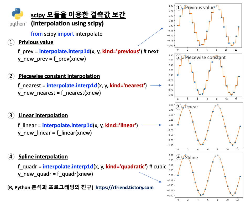
1. 이전 값/ 이후 값을 이용하여 결측값 채우기 (Imputation using the previous/next values)
2. Piecewise Constant Interpolation
3. 선형 보간법 (Linear Interpolation)
4. 스플라인 보간법 (Spline Interpolation)
[ Python scipy 모듈을 이용한 결측값 보간 (Interpolation using Python scipy module) ]
먼저 '0.5'로 동일한 간격을 가지는 x 값들에 대한 사인 함수 (sine function) 의 y값을 계산해서 예제 데이터로 사용하겠습니다. 아래 예졔의 점과 점 사이의 값들이 비어있는 결측값이라고 간주하고, 이들 값을 채워보겠습니다.
import numpy as np
from scipy import interpolate
import matplotlib.pyplot as plt

## generating the original data with missing values
x = np.arange(0, 4*np.pi, 0.5)
y = np.sin(x)

plt.plot(x, y, "o")
plt.show()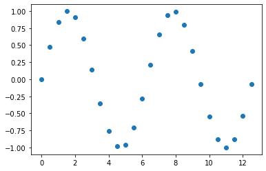
1. 이전 값/ 다음 값을 이용하여 결측값 채우기 (Imputation using the previous/next values)
데이터 포인트 사이의 값을 채우는 가장 간단한 방법은 이전 값(previous value) 나 또는 다음 값(next value)을 이용하는 것입니다. 함수를 추정하는 절차가 필요없으므로 연산 상 부담이 적지만, 데이터 추정 오차는 단점이 될 수 있습니다.
## Interpolation using the previous value
f_prev = interpolate.interp1d(
    x, y, kind='previous') # next
y_new_prev = f_prev(xnew)

plt.plot(x, y, "o", xnew, y_new_prev, '-')
plt.show()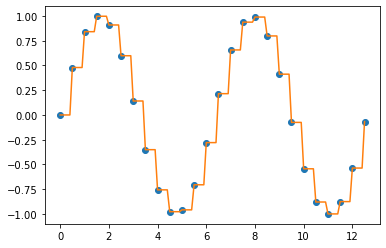
2. Piecewise Constant Interpolation
위 1번의 이전 값 또는 다음 값을 이용한 사이값 채우기를 합쳐놓은 방법입니다. Piecewise Constant Interpolation은 특정 데이터 포인트를 기준으로 가장 가까운 값 (nearest value) 을 가져다가 사이값을 보간합니다. ("최근접 이웃 보간"이라고도 함)
간단한 문제에서는 아래 3번에서 소개하는 Linear Interpolation 이 주로 사용되고, Piecewise Constant Interpolation 은 잘 사용되지 않는 편입니다. 하지만 다차원의 다변량 보간 (in higher-dimensional multivariate interpolation)의 경우, 속도와 단순성(speed and simplicity) 측면에서 선호하는 선택이 될 수 있습니다.
## Piecewise Constant Interpolation
f_nearest = interpolate.interp1d(
    x, y, kind='nearest')

y_new_nearest = f_nearest(xnew)

plt.plot(x, y, "o", xnew, y_new_nearest)
plt.show()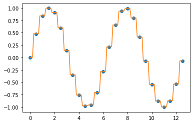
3. Linear Interpolation
선형 보간법은 가장 쉬운 보간법 중의 하나로서, 연산이 빠르고 쉽습니다. 하지만 추정값이 정확한 편은 아니며, 데이터 포인트 Xk 에서 미분 가능하지 않다는 단점도 있습니다.
일반적으로, 선형 보간법은 두 개의 데이터 포인트, 가령 (Xa, Ya)와 (Xb, Yb), 를 사용해서 다음의 공식으로 두 값 사이의 값을 보간합니다.
Y = Ya + (Yb - Ya) * (X - Xa) / (Xb- Xa) at the point (x, y)
## Linear Interpolation
f_linear = interpolate.interp1d(
    x, y, kind='linear')

y_new_linear = f_linear(xnew)

plt.plot(x, y, "o", xnew, y_new_linear, '-')
plt.show()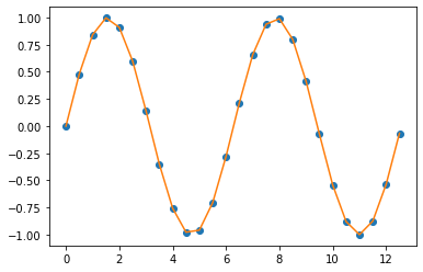
4. Spline Interpolation
다항식 보간법(Polynomial Interpolation)은 선형 보간법을 일반화(generalization of linear interpolation)한 것입니다. 선형 보간법에서는 선형 함수를 사용했다면, 다항식 보간법에서는 더 높은 차수의 다항식 함수를 사용해서 보간하는 것으로 대체한 것입니다.
일반적으로, 만약 우리가 n개의 데이터 포인트를 가지고 있다면 모든 데이터 포인트를 통과하는 n-1 차수의 다차항 함수가 존재합니다. 보간 오차는 데이터 포인트 간의 거리의 n 차승에 비례(interpolation error is proportional to the distance between the data points to the power n)하며, 다차항 함수는 미분가능합니다. 따라서 선형 보간법의 대부분의 문제를 다항식 보간법은 극복합니다. 하지만 다항식 보간법은 선형 보간법에 비해 복잡하고 연산에 많은 비용이 소요됩니다. 그리고 끝 점(end point) 에서는 진동하면서 변동성이 큰 값을 추정하는 문제가 있습니다.
스플라인 보간법은 각 데이터 포인트 구간별로 낮은 수준의 다항식 보간을 사용 (Spline interpolation uses low-degree polynomials in each of the intervals) 합니다. 그리고 이들이 함께 부드럽게 연결되어서 적합될 수 있도록 다항식 항목을 선택(, and chooses the polynomial pieces such that they fit smoothly together)합니다. 이렇게 적합된 함수를 스플라인(Spline) 이라고 합니다.
스플라인 보간법(Spline Interpolation)은 다항식 보간법의 장점은 살리고 단점은 피해간 보간법입니다. 스플라인 보간법은 다항식 보간법처럼 선형 보간법보다 보간 오차가 더 작은 반면에, 고차항의 다항식 보간법보다는 보간 함수가 부드럽고 평가하기가 쉽습니다.
## Spline Interpolation
f_quadr = interpolate.interp1d(
    x, y, kind='quadratic') # cubic

y_new_quadr = f_quadr(xnew)

plt.plot(x, y, "o", xnew, y_new_quadr)
plt.show()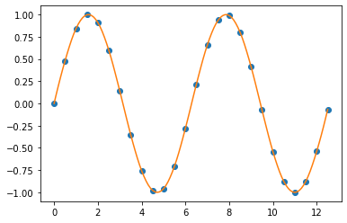
[ Reference ]
1. 보간법(interpolation): https://en.wikipedia.org/wiki/Interpolation
2. scipy 모듈: https://docs.scipy.org/doc/scipy/reference/generated/scipy.interpolate.interp1d.html
이번 포스팅이 많은 도움이 되었기를 바랍니다.
행복한 데이터 과학자 되세요! :-)