지난번 포스팅에서는 시계열 패턴 별 지수평활법 모델을 설정하는 방법 (https://rfriend.tistory.com/511), 그리고 시계열 데이터 예측 모델의 성능, 모델 적합도 (goodness-of-fit of time series model)를 평가하는 지표 (https://rfriend.tistory.com/667) 에 대해서 소개하였습니다.  


이번 포스팅에서는 간단한 시계열 예제 데이터에 대해 앞서 소개한 이론들을 Python 코드로 실습하여 

(1) 지수평활법(Exponential Smoothing) 기법으로 시계열 예측 모델을 만들고, 

(2) 모델 적합도를 평가하는 여러 지표들로 성능을 평가해서 최적의 모델을 선택

해보겠습니다. 


예제로 사용할 시계열 데이터는 1991년 7월부터 2008년 6월까지 월 단위(monthly)로 집계된 약 판매량 시계열 데이터셋 (drug sales time series dataset) 입니다. 


import pandas as pd
import numpy as np
import matplotlib.pyplot as plt

## getting drug sales dataset
file_path = 'https://raw.githubusercontent.com/selva86/datasets/master/a10.csv'
df = pd.read_csv(file_path, 
                 parse_dates=['date'], 
                 index_col='date')
                 
df.head(12)

# [Out]
#             value
# date	
# 1991-07-01	3.526591
# 1991-08-01	3.180891
# 1991-09-01	3.252221
# 1991-10-01	3.611003
# 1991-11-01	3.565869
# 1991-12-01	4.306371
# 1992-01-01	5.088335
# 1992-02-01	2.814520
# 1992-03-01	2.985811
# 1992-04-01	3.204780
# 1992-05-01	3.127578
# 1992-06-01	3.270523


## time series plot
df.plot(figsize=[12, 8])
plt.title('Drug Sales', fontsize=14)
plt.show()

drug sales time series plot


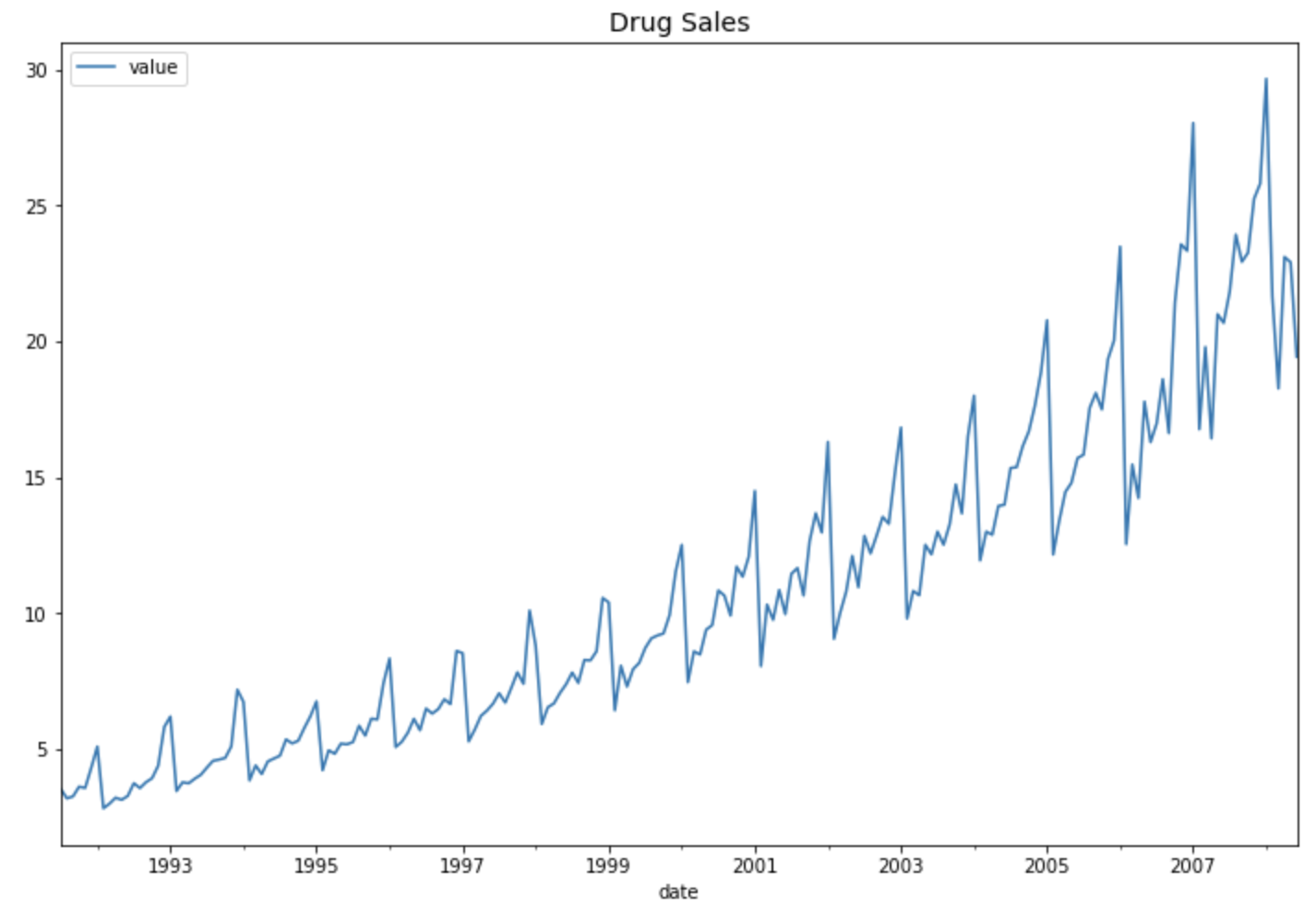
위의 약 판매량 시도표 (time series plot of drug sales) 를 보면 세 가지를 알 수 있습니다. 


(a) 선형 추세가 존재합니다. (linear or quadratic trend)

(b) 1년 단위의 계절성이 존재합니다. (seasonality of a year, ie. 12 months)

(c) 분산이 시간의 흐름에 따라 점점 커지고 있습니다. (increasing variation)


우리가 관찰한 이들 세가지의 시계열 데이터의 패턴으로 부터 "Multiplicative Winters' method with Linear / Quadratic Trend" 모델이 적합할 것이라고 판단해볼 수 있습니다. 

* 참조: 시계열 패턴 별 지수평활법 모델을 설정하는 방법 (https://rfriend.tistory.com/511)


그럼, 실제로 다양한 지수평활법으로 위의 약 판매량 시계열 데이터에 대한 예측 모델을 만들어 예측을 해보고, 다양한 평가지표로 모델 간 비교를 해봐서 가장 우수한 모델이 무엇인지, 과연 앞서 말한 "Multiplicative Winters' method with Linear Trend" 모델이 가장 우수할 것인지 확인해보겠습니다. 보는게 믿는거 아니겠습니까!


이제 월 단위로 시간 순서대로 정렬된 시계열 데이터를 제일 뒤 (최근)의 12개월치는 시계열 예측 모델의 성능을 평가할 때 사용할 test set으로 따로 떼어놓고, 나머지 데이터는 시계열 예측모형 훈련에 사용할 training set 으로 분할 (splitting between the training and the test set)을 해보겠습니다. 


## split between the training and the test data sets. 
## The last 12 periods form the test data
df_train = df.iloc[:-12]
df_test = df.iloc[-12:]


(1) 지수평활법 기법으로 시계열 예측모형 적합하기
       (training the exponential smoothing models in Python)


Python의 statsmodels 라이브러리는 시계열 데이터 분석을 위한 API를 제공합니다. 아래의 코드는 순서대로 


(a) Simple Exponential Smoothing 

-- 추세 요소의 유형 (type of trend components)에 따라서 

(b) Holt's (trend=None)

(c) Exponential trend (exponential=True)

(d) Additive damped trend (damped_trend=True)

(e) Multiplicative damped trend (exponential=True, damped_trend=True)


로 구분할 수 있습니다. 


## exponential smoothing in Python
from statsmodels.tsa.api import ExponentialSmoothing, SimpleExpSmoothing, Holt

# Simple Exponential Smoothing
fit1 = SimpleExpSmoothing(df_train, 
                          initialization_method="estimated").fit()

# Trend
fit2 = Holt(df_train, 
            initialization_method="estimated").fit()

# Exponential trend
fit3 = Holt(df_train,
            exponential=True, 
            initialization_method="estimated").fit()

# Additive damped trend
fit4 = Holt(df_train,
            damped_trend=True, 
            initialization_method="estimated").fit()

# Multiplicative damped trend
fit5 = Holt(df_train,
            exponential=True, 
            damped_trend=True, 
            initialization_method="estimated").fit()


statsmodels.tsa.api 메소드를 사용해서 적합한 시계열 데이터 예측 모델에 대해서는 model_object.summary() 메소드를 사용해서 적합 결과를 조회할 수 있습니다. 그리고 model_object.params['parameter_name'] 의 방식으로 지수평활법 시계열 적합 모델의 속성값(attributes of the fitted exponential smoothing results)에 대해서 조회할 수 있습니다. 


## accessing the results of SimpleExpSmoothing Model
print(fit1.summary())

#                        SimpleExpSmoothing Model Results                       
# ==============================================================================
# Dep. Variable:                  value   No. Observations:                  192
# Model:             SimpleExpSmoothing   SSE                            692.196
# Optimized:                       True   AIC                            250.216
# Trend:                           None   BIC                            256.731
# Seasonal:                        None   AICC                           250.430
# Seasonal Periods:                None   Date:                 Thu, 29 Jul 2021
# Box-Cox:                        False   Time:                         19:26:46
# Box-Cox Coeff.:                  None                                         
# ==============================================================================
#                        coeff                 code              optimized      
# ------------------------------------------------------------------------------
# smoothing_level            0.3062819                alpha                 True
# initial_level              3.4872869                  l.0                 True
# ------------------------------------------------------------------------------


## getting all results by models
params = ['smoothing_level', 'smoothing_trend', 'damping_trend', 'initial_level', 'initial_trend']
results=pd.DataFrame(index=[r"$\alpha$",r"$\beta$",r"$\phi$",r"$l_0$","$b_0$","SSE"],
                     columns=['SES', "Holt's","Exponential", "Additive", "Multiplicative"])

results["SES"] =            [fit1.params[p] for p in params] + [fit1.sse]
results["Holt's"] =         [fit2.params[p] for p in params] + [fit2.sse]
results["Exponential"] =    [fit3.params[p] for p in params] + [fit3.sse]
results["Additive"] =       [fit4.params[p] for p in params] + [fit4.sse]
results["Multiplicative"] = [fit5.params[p] for p in params] + [fit5.sse]

results
# [Out]
#      SES	Holt's	Exponential	Additive	Multiplicative
# 𝛼 	0.306282	0.053290	1.655513e-08	0.064947	0.040053
# 𝛽 	NaN	0.053290	1.187778e-08	0.064947	0.040053
# 𝜙 	NaN	NaN	NaN	0.995000	0.995000
# 𝑙0 	3.487287	3.279317	3.681273e+00	3.234974	3.382898
# 𝑏0 	NaN	0.045952	1.009056e+00	0.052515	1.016242
# SSE  692.195826	631.551871	5.823167e+02	641.058197	621.344891


계절성(seasonality)을 포함한 지수평활법에 대해서는 statsmodels.tsa.holtwinters 내의 메소드를 사용해서 시계열 예측 모델을 적합해보겠습니다. 


seasonal_periods 에는 계절 주기를 입력해주는데요, 이번 예제에서는 월 단위 집계 데이터에서 1년 단위로 계절성이 나타나고 있으므로 seasonal_periods = 12 를 입력해주었습니다. 

trend = 'add' 로 일단 고정을 했으며, 대신에 계절성의 경우 (f) seasonal = 'add' (or 'additive'), (g) seasonal = 'mul' (or 'multiplicative') 로 구분해서 모델을 각각 적합해보았습니다. 


위의 시계열 시도표를 보면 시간이 흐름에 따라 분산이 점점 커지고 있으므로  seasonal = 'mul' (or 'multiplicative') 가 더 적합할 것이라고 우리는 예상할 수 있습니다. 실제 그런지 데이터로 확인해보겠습니다. 


## Holt's Winters's method for time series data with Seasonality
from statsmodels.tsa.holtwinters import ExponentialSmoothing as HWES

# additive model for fixed seasonal variation
fit6 = HWES(df_train, 
             seasonal_periods=12, 
             trend='add', 
             seasonal='add').fit(optimized=True, use_brute=True)

# multiplicative model for increasing seasonal variation
fit7 = HWES(df_train, 
             seasonal_periods=12, 
             trend='add', 
             seasonal='mul').fit(optimized=True, use_brute=True)


(2) 지수평활법 적합 모델로 예측하여 모델 간 성능 평가/비교하고 최적 모델 선택하기

     (forecasting using the exponential smoothing models, model evaluation/ model comparison and best model selection)


(2-1) 향후 12개월 약 판매량 예측하기 (forecasting the drug sales for the next 12 months) 


forecast() 함수를 사용하며, 괄호 안에는 예측하고자 하는 기간을 정수로 입력해줍니다. 


## forecasting for 12 months
forecast_1 = fit1.forecast(12)
forecast_2 = fit2.forecast(12)
forecast_3 = fit3.forecast(12)
forecast_4 = fit4.forecast(12)
forecast_5 = fit5.forecast(12)
forecast_6 = fit6.forecast(12)
forecast_7 = fit7.forecast(12


y_test = df_test['value']

t_p = pd.DataFrame({'test': y_test, 
                    'f1': forecast_1, 
                    'f2': forecast_2, 
                    'f3': forecast_3, 
                    'f4': forecast_4, 
                    'f5': forecast_5, 
                    'f6': forecast_6, 
                    'f7': forecast_7})
                    
                    
print(t_p)

#                  test        f1         f2         f3         f4         f5  \
# 2007-07-01  21.834890  20.15245  20.350267  20.970823  20.454211  20.261185   
# 2007-08-01  23.930204  20.15245  20.511013  21.160728  20.616026  20.421627   
# 2007-09-01  22.930357  20.15245  20.671760  21.352352  20.777032  20.582528   
# 2007-10-01  23.263340  20.15245  20.832507  21.545711  20.937233  20.743882   
# 2007-11-01  25.250030  20.15245  20.993254  21.740821  21.096633  20.905686   
# 2007-12-01  25.806090  20.15245  21.154000  21.937699  21.255236  21.067932   
# 2008-01-01  29.665356  20.15245  21.314747  22.136359  21.413046  21.230618   
# 2008-02-01  21.654285  20.15245  21.475494  22.336818  21.570067  21.393736   
# 2008-03-01  18.264945  20.15245  21.636241  22.539092  21.726303  21.557283   
# 2008-04-01  23.107677  20.15245  21.796987  22.743198  21.881758  21.721254   
# 2008-05-01  22.912510  20.15245  21.957734  22.949152  22.036435  21.885642   
# 2008-06-01  19.431740  20.15245  22.118481  23.156972  22.190339  22.050443   

#                    f6         f7  
# 2007-07-01  20.882394  21.580197  
# 2007-08-01  22.592307  22.164134  
# 2007-09-01  21.388974  22.136953  
# 2007-10-01  25.178594  24.202879  
# 2007-11-01  26.776556  25.322929  
# 2007-12-01  26.424404  27.549045  
# 2008-01-01  30.468546  31.194773  
# 2008-02-01  19.065461  18.181477  
# 2008-03-01  21.834584  21.034783  
# 2008-04-01  19.061426  20.085947  
# 2008-05-01  23.452042  23.076423  
# 2008-06-01  22.353486  22.598155


(2-2) 모델 간 모델적합도/성능 평가하고 비교하기


Python의 scikit-learn 라이브러리의 metrics 메소드에 이미 정의되어 있는 MSE, MAE 지표는 가져다가 쓰구요, 없는 지표는 모델 적합도 (goodness-of-fit of time series model)를 평가하는 지표 (https://rfriend.tistory.com/667) 포스팅에서 소개했던 수식대로 Python 사용자 정의 함수(User Defined Funtion)을 만들어서 사용하겠습니다. 


아래의 모델 성능 평가 지표 중에서 AIC, SBC, APC, Adjsted-R2 지표는 모델 적합에 사용된 모수의 개수 (the number of parameters) 를 알아야지 계산할 수 있으며, 모수의 개수는 지수평활법 모델 종류별로 다르므로, 적합된 모델 객체로부터 모수 개수를 세는 사용자 정의함수를 먼저 정의해보겠습니다. 


## UDF for counting the number of parameters in model
def num_params(model):
    n_params = 0

    for p in list(model.params.values()):
        if isinstance(p, np.ndarray):
            n_params += len(p)
            #print(p)
        elif p in [np.nan, False, None]:
            pass
        elif np.isnan(float(p)):
            pass
        else:
            n_params += 1
            #print(p)
    
    return n_params
    

num_params(fit1)
[Out] 2

num_params(fit7)
[Out] 17


이제 각 지표별로 Python을 사용해서 지수평활법 모델별로 성능을 평가하는 사용자 정의함수를 정의해보겠습니다. MSE와 MAE는 scikit-learn.metrics 에 있는 메소드를 가져다가 사용하며, 나머지는 공식에 맞추어서 정의해주었습니다.

(혹시 sklearn 라이브러리에 모델 성능 평가 지표 추가로 더 있으면 그거 가져다 사용하시면 됩니다. 저는 sklearn 튜토리얼 찾아보고 없는거 같아서 아래처럼 정의해봤어요. 혹시 코드 잘못된거 있으면 댓글에 남겨주시면 감사하겠습니다.)


## number of observations in training set
T = df_train.shape[0]
print(T)
[Out] 192


## evaluation metrics
from sklearn.metrics import mean_squared_error as MSE
from sklearn.metrics import mean_absolute_error as MAE

# Mean Absolute Percentage Error
def SSE(y_test, y_pred):
    y_test, y_pred = np.array(y_test), np.array(y_pred)
    return np.sum((y_test - y_pred)**2)

def ME(y_test, y_pred):
    y_test, y_pred = np.array(y_test), np.array(y_pred)
    return np.mean(y_test - y_pred)

def RMSE(y_test, y_pred):
    y_test, y_pred = np.array(y_test), np.array(y_pred)
    return np.sqrt(np.mean((y_test - y_pred)**2))   
    #return np.sqrt(MSE(y_test - y_pred))

def MPE(y_test, y_pred): 
    y_test, y_pred = np.array(y_test), np.array(y_pred)
    return np.mean((y_test - y_pred) / y_test) * 100

def MAPE(y_test, y_pred): 
    y_test, y_pred = np.array(y_test), np.array(y_pred)
    return np.mean(np.abs((y_test - y_pred) / y_test)) * 100

def AIC(y_test, y_pred, T, model):
    y_test, y_pred = np.array(y_test), np.array(y_pred)
    sse = np.sum((y_test - y_pred)**2)
    #T = len(y_train) # number of observations
    k = num_params(model) # number of parameters
    return T * np.log(sse/T) + 2*k

def SBC(y_test, y_pred, T, model):
    y_test, y_pred = np.array(y_test), np.array(y_pred)
    sse = np.sum((y_test - y_pred)**2)
    #T = len(y_train) # number of observations
    k = num_params(model) # number of parameters
    return T * np.log(sse/T) + k * np.log(T)

def APC(y_test, y_pred, T, model):
    y_test, y_pred = np.array(y_test), np.array(y_pred)
    sse = np.sum((y_test - y_pred)**2)
    #T = len(y_train) # number of observations
    k = num_params(model) # number of parameters
    return ((T+k)/(T-k)) * sse / T

def ADJ_R2(y_test, y_pred, T, model):
    y_test, y_pred = np.array(y_test), np.array(y_pred)
    sst = np.sum((y_test - np.mean(y_test))**2)
    sse = np.sum((y_test - y_pred)**2)
    #T = len(y_train) # number of observations
    k = num_params(model) # number of parameters
    r2 = 1 - sse/sst
    return 1 - ((T - 1)/(T - k)) * (1 - r2)
    

## Combining all metrics together
def eval_all(y_test, y_pred, T, model):
    sse = SSE(y_test, y_pred)
    mse = MSE(y_test, y_pred)
    rmse = RMSE(y_test, y_pred)
    me = ME(y_test, y_pred)
    mae = MAE(y_test, y_pred)
    mpe = MPE(y_test, y_pred)
    mape = MAPE(y_test, y_pred)
    aic = AIC(y_test, y_pred, T, model)
    sbc = SBC(y_test, y_pred, T, model)
    apc = APC(y_test, y_pred, T, model)
    adj_r2 = ADJ_R2(y_test, y_pred, T, model)
    
    return [sse, mse, rmse, me, mae, mpe, mape, aic, sbc, apc, adj_r2]


위에서 정의한 시계열 예측 모델 성능평가 지표 사용자 정의 함수를 모델 성능 평가를 위해 따로 떼어놓았던 'test set' 에 적용하여 각 지수평활법 모델별/ 모델 성능평가 지표 별로 비교를 해보겠습니다. 

모델 성능평가 지표 중에서 실제값과 예측값의 차이인 잔차(residual)를 기반으로 한 MSE, RMSE, ME, MAE, MPE, MAPE, AIC, SBC, APC 는 낮을 수록 상대적으로 더 좋은 모델이라고 평가할 수 있으며, 실제값과 평균값의 차이 중에서 시계열 예측 모델이 설명할 수 있는 부분의 비중 (모델의 설명력) 을 나타내는 Adjusted-R2 는 값이 높을 수록 상대적으로 더 좋은 모델이라고 평가합니다. (Ajd.-R2 가 음수가 나온 값이 몇 개 보이는데요, 이는 예측 모델이 불량이어서 예측값이 실제값과 차이가 큼에 따라 SSE가 SST보다 크게 되었기 때문입니다.)


eval_all_df = pd.DataFrame(
    {'SES': eval_all(y_test, forecast_1, T, fit1), 
    "Holt's": eval_all(y_test, forecast_2, T, fit2), 
    'Exponential': eval_all(y_test, forecast_3, T, fit3), 
    'Trend_Add': eval_all(y_test, forecast_4, T, fit4), 
    'Trend_Mult': eval_all(y_test, forecast_5, T, fit5), 
    'Trend_Season_Add': eval_all(y_test, forecast_6, T, fit6), 
    'Trend_Season_Mult': eval_all(y_test, forecast_7, T, fit7)}
    , index=['SSE', 'MSE', 'RMSE', 'ME', 'MAE', 'MPE', 'MAPE', 'AIC', 'SBC', 'APC', 'Adj_R2'])


print(eval_all_df)
#                SES      Holt's  Exponential   Trend_Add  Trend_Mult  \
# SSE     205.629692  155.645609   130.567477  150.867568  159.856508   
# MSE      17.135808   12.970467    10.880623   12.572297   13.321376   
# RMSE      4.139542    3.601454     3.298579    3.545744    3.649846   
# ME        3.018502    1.936578     1.123475    1.841425    2.019134   
# MAE       3.453205    2.946251     2.576567    2.878085    3.004307   
# MPE      11.739201    6.900165     3.313095    6.486233    7.259990   
# MAPE     14.079695   12.280881    10.960354   12.010763   12.510302   
# AIC      17.167661  -32.303428   -66.036202  -36.289847  -25.178006   
# SBC      23.682652  -19.273447   -53.006220  -20.002370   -8.890530   
# APC       1.093535    0.845150     0.708977    0.827788    0.877109   
# Adj_R2   -1.146688   -0.642161    -0.377571   -0.600262   -0.695608   

#         Trend_Season_Add  Trend_Season_Mult  
# SSE            56.743149          48.994715  
# MSE             4.728596           4.082893  
# RMSE            2.174533           2.020617  
# ME             -0.118946          -0.089689  
# MAE             1.863421           1.641140  
# MPE            -0.847971          -0.607618  
# MAPE            8.538100           7.461092  
# AIC          -200.040404        -228.230323  
# SBC          -144.662983        -172.852902  
# APC             0.352956           0.304759  
# Adj_R2          0.356850           0.444674


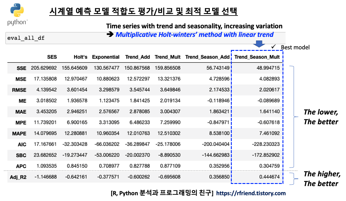
시계열 모델 성능 지표별로 보면 전반적으로 7번째 지수평활법 시계열 예측 모델인 "Multiplicative Winters' method with Linear Trend" 모델이 상대적으로 가장 우수함을 알 수 있습니다. 역시 시도표를 보고서 우리가 예상했던대로 결과가 나왔습니다. 

MAPE (Mean Absolute Percentage Error)  지표에 대해서만 옆으로 누운 막대그래프로 모델 간 성능을 비교해서 시각화를 해보면 아래와 같습니다. (MAPE 값이 작을수록 상대적으로 더 우수한 모델로 해석함.)


# horizontal bar chart
eval_all_df.loc['MAPE', :].plot(kind='barh', figsize=[8, 6])
plt.title('Mean Absolute Percentage Error (MAPE)', fontsize=16)
plt.show()

Mean Absolute Percentage Error (MAPE)


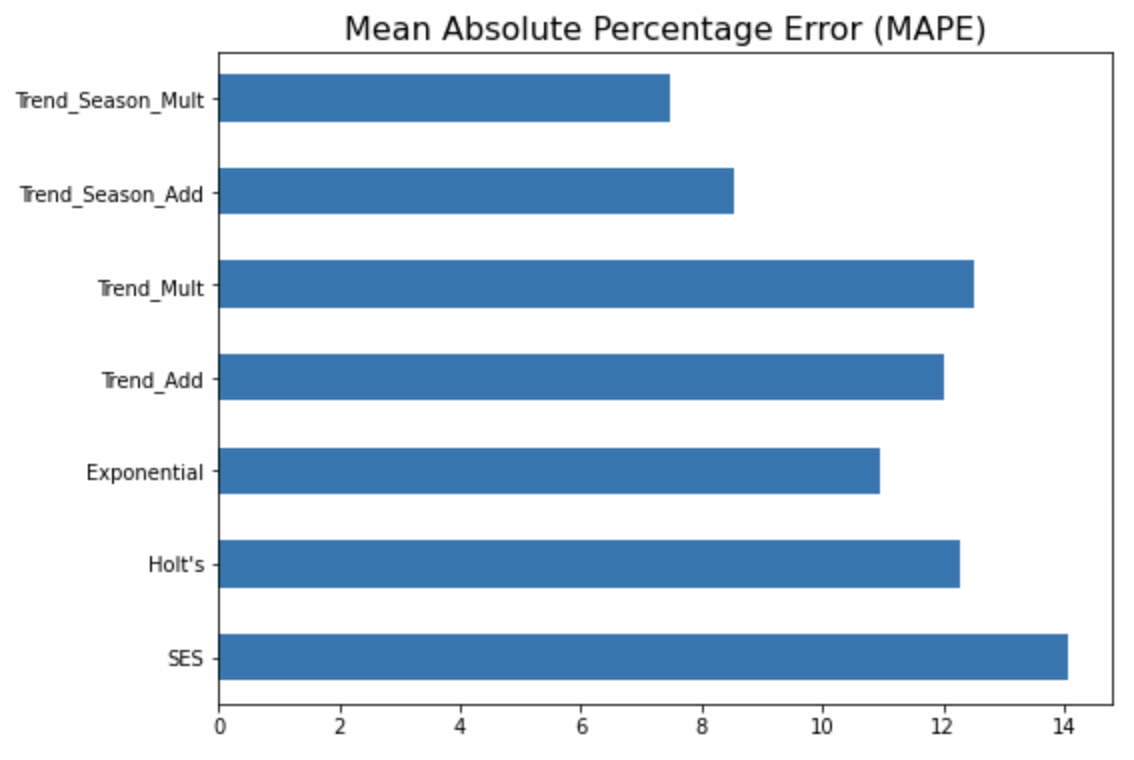
아래의 시도표는 실제값과 예측값을 시간의 흐름에 따라 선그래프로 시각화해 본 것입니다. 

예상했던 대로 4번째의 "1차 선형 추세만 반영하고 계절성은 없는 이중 지수 평활법 모델" 보다는, 7번째의 "선형추세+계절성까지 반영한 multiplicative holt-winters method exponential smoothing with linear trend 지수평활법 모델" 이 더 실제값을 잘 모델링하여 근접하게 예측하고 있음을 눈으로 확인할 수 있습니다. 


# 1차 선형 추세는 있고 계절성은 없는 이중 지수 평활법
plt.rcParams['figure.figsize']=[12, 8]
past, = plt.plot(df_train.index, df_train, 'b.-', label='Sales History')
test, = plt.plot(df_test.index, df_test, 'r.-', label='y_test')
pred, = plt.plot(df_test.index, forecast_4, 'y.-', label='y_pred')
plt.title('Two Parameter Exponential Smoothing', fontsize=14)
plt.legend(handles=[past, test, pred])
plt.show()


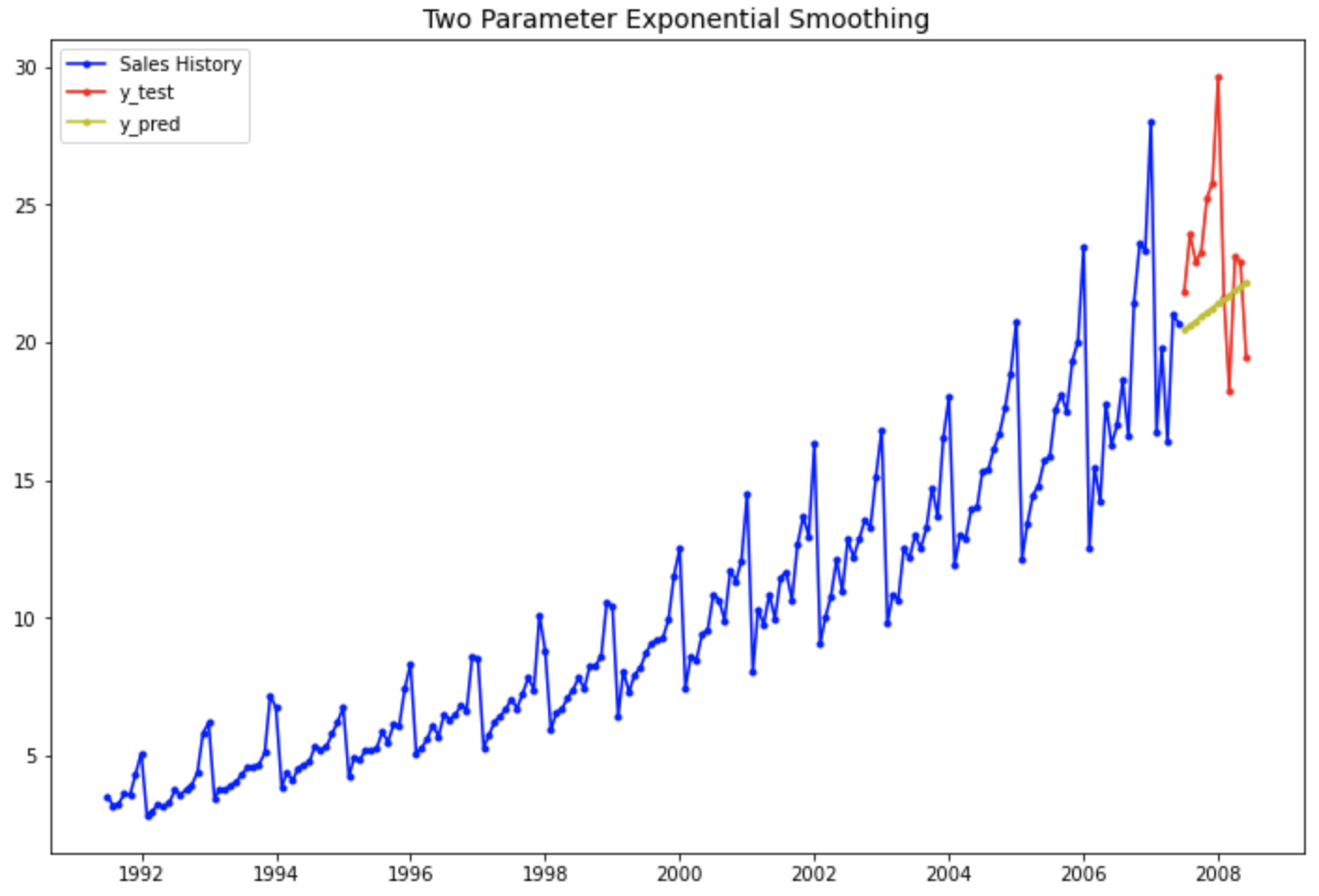
# 1차 선형 추세와 확산계절변동이 있는 승법 윈터스 지수평활법
plt.rcParams['figure.figsize']=[12, 8]
past, = plt.plot(df_train.index, df_train, 'b.-', label='Sales History')
test, = plt.plot(df_test.index, df_test, 'r.-', label='y_test')
pred, = plt.plot(df_test.index, forecast_7, 'y.-', label='y_pred')
plt.title('Multiplicative Winters Method Exponential Smoothing with Linear Trend', fontsize=14)
plt.legend(handles=[past, test, pred])
plt.show()


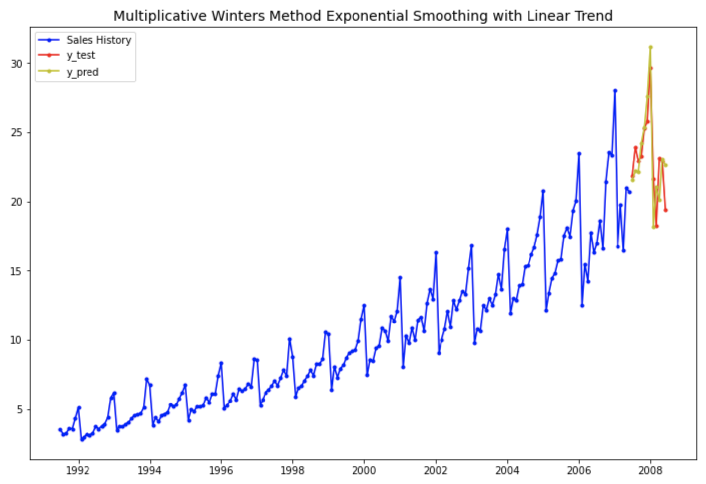
적합된 statsmodels.tsa 시계열 예측 모델에 대해 summary() 메소드를 사용해서 적합 결과를 조회할 수 있으며, model.params['param_name'] 으로 적합된 모델의 속성값에 접근할 수 있습니다. 


#print out the training summary
print(fit7.summary())

#                        ExponentialSmoothing Model Results                       
# ================================================================================
# Dep. Variable:                    value   No. Observations:                  192
# Model:             ExponentialSmoothing   SSE                             75.264
# Optimized:                         True   AIC                           -147.808
# Trend:                         Additive   BIC                            -95.688
# Seasonal:                Multiplicative   AICC                          -143.854
# Seasonal Periods:                    12   Date:                 Thu, 29 Jul 2021
# Box-Cox:                          False   Time:                         19:40:52
# Box-Cox Coeff.:                    None                                         
# =================================================================================
#                           coeff                 code              optimized      
# ---------------------------------------------------------------------------------
# smoothing_level               0.2588475                alpha                 True
# smoothing_trend               0.0511336                 beta                 True
# smoothing_seasonal           3.3446e-16                gamma                 True
# initial_level                 2.1420252                  l.0                 True
# initial_trend                 0.0466926                  b.0                 True
# initial_seasons.0             1.4468847                  s.0                 True
# initial_seasons.1             1.4713123                  s.1                 True
# initial_seasons.2             1.4550909                  s.2                 True
# initial_seasons.3             1.5754307                  s.3                 True
# initial_seasons.4             1.6324776                  s.4                 True
# initial_seasons.5             1.7590615                  s.5                 True
# initial_seasons.6             1.9730448                  s.6                 True
# initial_seasons.7             1.1392096                  s.7                 True
# initial_seasons.8             1.3057795                  s.8                 True
# initial_seasons.9             1.2354317                  s.9                 True
# initial_seasons.10            1.4064560                 s.10                 True
# initial_seasons.11            1.3648905                 s.11                 True
# ---------------------------------------------------------------------------------


print('Smoothing Level: %.3f' %(fit7.params['smoothing_level']))
print('Smoothing Trend: %.3f' %(fit7.params['smoothing_trend']))
print('Smoothing Seasonality: %.3f' %(fit7.params['smoothing_seasonal']))
print('Initial Level: %.3f' %(fit7.params['initial_level']))
print('Initial Trend: %.3f' %(fit7.params['initial_trend']))
print('Initial Seasons:', fit7.params['initial_seasons'])

# Smoothing Level: 0.259
# Smoothing Trend: 0.051
# Smoothing Seasonality: 0.000
# Initial Level: 2.142
# Initial Trend: 0.047
# Initial Seasons: [1.44688473 1.47131227 1.45509092 1.5754307  1.63247755 1.75906148
#  1.97304481 1.13920961 1.30577953 1.23543175 1.40645604 1.36489053]


[Reference]

* Exponential Smoothing
https://www.statsmodels.org/stable/examples/notebooks/generated/exponential_smoothing.html
* Holt-Winters 
https://www.statsmodels.org/devel/generated/statsmodels.tsa.holtwinters.ExponentialSmoothing.html


Exponential smoothing — statsmodels

Exponential smoothing Let us consider chapter 7 of the excellent treatise on the subject of Exponential Smoothing By Hyndman and Athanasopoulos [1]. We will work through all the examples in the chapter as they unfold. [1] [Hyndman, Rob J., and George Athan

www.statsmodels.org


statsmodels.tsa.holtwinters.ExponentialSmoothing — statsmodels

An dictionary containing bounds for the parameters in the model, excluding the initial values if estimated. The keys of the dictionary are the variable names, e.g., smoothing_level or initial_slope. The initial seasonal variables are labeled initial_season

www.statsmodels.org


* 시계열 패턴 별 지수평활법 모델을 설정하는 방법
   :
https://rfriend.tistory.com/511

* 시계열 데이터 예측 모델의 성능, 모델 적합도 (goodness-of-fit of time series model)를 평가하는 지표
   :
https://rfriend.tistory.com/667


이번 포스팅이 많은 도움이 되었기를 바랍니다. 

행복한 데이터 과학자 되세요! :-)


728x90
반응형
Posted by Rfriend
,

지난번 포스팅에서는 시계열 자료의 구성 요인 (time series component factors)으로서 추세 요인, 순환 요인, 계절 요인, 불규칙 요인에 대해서 소개하였습니다. 


지난번 포스팅에서는 가법 모형으로 가상의 시계열 자료를 만들었다면(time series composition), ==> 이번 포스팅에서는 반대로 시계열 분해(time series decomposition)를 통해 시계열 자료를 추세(순환)(Trend), 계절성(Seasonality), 잔차(Residual)로 분해를 해보겠습니다. 


시계열 분해는 직관적으로 이해하기 쉽고 구현도 쉬워서 시계열 자료 분석의 고전적인 방법론이지만 지금까지도 꾸준히 사용되는 방법론입니다. 시계열 분해의 순서와 방법은 대략 아래와 같습니다. 


(1) 시도표 (time series plot)를 보고 시계열의 주기적 반복/계절성이 있는지, 가법 모형(additive model, y = t + s + r)과 승법 모형(multiplicative model, y = t * s * r) 중 무엇이 더 적합할지 판단을 합니다. 


(가법 모형을 가정할 시)

(2) 시계열 자료에서 추세(trend)를 뽑아내기 위해서 중심 이동 평균(centered moving average)을 이용합니다. 


(3) 원 자료에서 추세 분해값을 빼줍니다(detrend). 그러면 계절 요인과 불규칙 요인만 남게 됩니다. 


(4) 다음에 계절 주기 (seasonal period) 로 detrend 이후 남은 값의 합을 나누어주면 계절 평균(average seasonality)을 구할 수 있습니다. (예: 01월 계절 평균 = (2020-01 + 2021-01 + 2022-01 + 2023-01)/4, 02월 계절 평균 = (2020-02 + 2021-02 + 2022-02 + 2023-02)/4). 


(5) 원래의 값에서 추세와 계절성 분해값을 빼주면 불규칙 요인(random, irregular factor)이 남게 됩니다. 


시계열 분해 후에 추세와 계절성을 제외한 잔차(residual, random/irregular factor) 가 특정 패턴 없이 무작위 분포를 띠고 작은 값이면 추세와 계절성으로 모형화가 잘 되는 것이구요, 시계열 자료의 특성을 이해하고 예측하는데 활용할 수 있습니다. 만약 시계열 분해 후의 잔차에 특정 패턴 (가령, 주기적인 파동을 그린다거나, 분산이 점점 커진다거나 등..) 이 존재한다면 잔차에 대해서만 다른 모형을 추가로 적합할 수도 있겠습니다. 


예제로 사용할 시계열 자료로서 '1차 선형 추세 + 4년 주기 순환 + 1년 단위 계절성 + 불규칙 noise' 의 가법 모형 (additive model)으로 시계열 데이터를 만들어보겠습니다. 


import numpy as np
import pandas as pd
import matplotlib.pyplot as plt


dates = pd.date_range('2020-01-01', periods=48, freq='M')
dates
[Out]:
DatetimeIndex(['2020-01-31', '2020-02-29', '2020-03-31', '2020-04-30', '2020-05-31', '2020-06-30', '2020-07-31', '2020-08-31', '2020-09-30', '2020-10-31', '2020-11-30', '2020-12-31', '2021-01-31', '2021-02-28', '2021-03-31', '2021-04-30', '2021-05-31', '2021-06-30', '2021-07-31', '2021-08-31', '2021-09-30', '2021-10-31', '2021-11-30', '2021-12-31', '2022-01-31', '2022-02-28', '2022-03-31', '2022-04-30', '2022-05-31', '2022-06-30', '2022-07-31', '2022-08-31', '2022-09-30', '2022-10-31', '2022-11-30', '2022-12-31', '2023-01-31', '2023-02-28', '2023-03-31', '2023-04-30', '2023-05-31', '2023-06-30', '2023-07-31', '2023-08-31', '2023-09-30', '2023-10-31', '2023-11-30', '2023-12-31'], dtype='datetime64[ns]', freq='M')


# additive model: trend + cycle + seasonality + irregular factor


timestamp = np.arange(len(dates))
trend_factor = timestamp*1.1
cycle_factor = 10*np.sin(np.linspace(0, 3.14*2, 48))
seasonal_factor = 7*np.sin(np.linspace(0, 3.14*8, 48))
np.random.seed(2004)
irregular_factor = 2*np.random.randn(len(dates))


df = pd.DataFrame({'timeseries': trend_factor + cycle_factor + seasonal_factor + irregular_factor, 
                   'trend': trend_factor, 
                   'cycle': cycle_factor, 
                   'trend_cycle': trend_factor + cycle_factor,
                   'seasonal': seasonal_factor, 
                   'irregular': irregular_factor},
                   index=dates)


df
[Out]:
  timeseries trend cycle trend_cycle seasonal irregular
2020-01-31 2.596119 0.0 0.000000 0.000000 0.000000 2.596119
2020-02-29 6.746160 1.1 1.332198 2.432198 3.565684 0.748278
2020-03-31 8.112100 2.2 2.640647 4.840647 6.136825 -2.865371
2020-04-30 8.255941 3.3 3.902021 7.202021 6.996279 -5.942358
2020-05-31 16.889655 4.4 5.093834 9.493834 5.904327 1.491495
2020-06-30 16.182357 5.5 6.194839 11.694839 3.165536 1.321981
2020-07-31 14.128087 6.6 7.185409 13.785409 -0.456187 0.798865
2020-08-31 11.943313 7.7 8.047886 15.747886 -3.950671 0.146099
2020-09-30 9.728095 8.8 8.766892 17.566892 -6.343231 -1.495567
2020-10-31 12.483489 9.9 9.329612 19.229612 -6.966533 0.220411
2020-11-30 12.141808 11.0 9.726013 20.726013 -5.646726 -2.937480
2020-12-31 15.143334 12.1 9.949029 22.049029 -2.751930 -4.153764
2021-01-31 21.774516 13.2 9.994684 23.194684 0.910435 -2.330604
2021-02-28 28.432892 14.3 9.862164 24.162164 4.318862 -0.048134
2021-03-31 32.350583 15.4 9.553832 24.953832 6.522669 0.874082
2021-04-30 30.596556 16.5 9.075184 25.575184 6.907169 -1.885797
2021-05-31 32.510523 17.6 8.434753 26.034753 5.365118 1.110653
2021-06-30 30.425519 18.7 7.643955 26.343955 2.326624 1.754939
2021-07-31 24.300958 19.8 6.716890 26.516890 -1.360813 -0.855119
2021-08-31 20.450917 20.9 5.670082 26.570082 -4.668691 -1.450475
2021-09-30 18.870881 22.0 4.522195 26.522195 -6.674375 -0.976939
2021-10-31 21.326310 23.1 3.293690 26.393690 -6.818438 1.751059
2021-11-30 22.902448 24.2 2.006469 26.206469 -5.060699 1.756678
2021-12-31 26.620578 25.3 0.683478 25.983478 -1.891426 2.528526
2022-01-31 27.626499 26.4 -0.651696 25.748304 1.805404 0.072791
2022-02-28 31.858923 27.5 -1.975253 25.524747 4.998670 1.335506
2022-03-31 35.930469 28.6 -3.263598 25.336402 6.797704 3.796363
2022-04-30 30.177870 29.7 -4.493762 25.206238 6.700718 -1.729087
2022-05-31 30.016165 30.8 -5.643816 25.156184 4.734764 0.125217
2022-06-30 26.591729 31.9 -6.693258 25.206742 1.448187 -0.063200
2022-07-31 21.118481 33.0 -7.623379 25.376621 -2.242320 -2.015820
2022-08-31 16.636031 34.1 -8.417599 25.682401 -5.307397 -3.738973
2022-09-30 17.682613 35.2 -9.061759 26.138241 -6.892132 -1.563496
2022-10-31 21.163298 36.3 -9.544375 26.755625 -6.554509 0.962182
2022-11-30 22.455672 37.4 -9.856844 27.543156 -4.388699 -0.698786
2022-12-31 26.919529 38.5 -9.993595 28.506405 -0.998790 -0.588086
2023-01-31 33.964623 39.6 -9.952191 29.647809 2.669702 1.647112
2023-02-28 37.459776 40.7 -9.733369 30.966631 5.593559 0.899586
2023-03-31 40.793766 41.8 -9.341031 32.458969 6.957257 1.377540
2023-04-30 43.838415 42.9 -8.782171 34.117829 6.380433 3.340153
2023-05-31 41.301780 44.0 -8.066751 35.933249 4.023975 1.344556
2023-06-30 39.217866 45.1 -7.207526 37.892474 0.545147 0.780245
2023-07-31 35.125502 46.2 -6.219813 39.980187 -3.085734 -1.768952
2023-08-31 33.841926 47.3 -5.121219 42.178781 -5.855940 -2.480916
2023-09-30 38.770511 48.4 -3.931329 44.468671 -6.992803 1.294643
2023-10-31 37.371216 49.5 -2.671356 46.828644 -6.179230 -3.278198
2023-11-30 46.587633 50.6 -1.363760 49.236240 -3.642142 0.993536
2023-12-31 46.403326 51.7 -0.031853 51.668147 -0.089186 -5.175634


  (1) Python을 이용한 시계열 분해 (Time series decomposition using Python)


Python의 statsmodels 라이브러리를 사용해서 가법 모형(additive model) 가정 하에 시계열 분해를 해보겠습니다. 


from statsmodels.tsa.seasonal import seasonal_decompose


ts = df.timeseries
result = seasonal_decompose(ts, model='additive')


plt.rcParams['figure.figsize'] = [12, 8]
result.plot()
plt.show()


원래의 시계열 구성요소(추세+순환, 계절성, 불규칙 요인)와 시계열 분해(time series decomposition)를 통해 분리한 추세(&순환), 계절성, 잔차(불규칙 요인)를 겹쳐서 그려보았습니다. (즉, 원래 데이터의 추세요인과 시계열 분해를 통해 분리한 추세를 겹쳐서 그려보고, 원래 데이터의 계절요인과 시계열 분해를 통해 분리한 계절을 겹쳐서 그려보고, 원래 데이터의 불규칙 요인과 시계열 분해를 통해 분리한 잔차를 겹쳐서 그려봄) 


원래의 데이터와 얼추 비슷하게, 그럴싸하게 시계열 분해를 한 것처럼 보이지요?   


# ground truth & timeseries decompostion all together
# -- observed data
plt.figure(figsize=(12, 12))
plt.subplot(4,1, 1)
result.observed.plot()
plt.grid(True)
plt.ylabel('Observed', fontsize=14)


# -- trend & cycle factor
plt.subplot(4, 1, 2)
result.trend.plot()        # from timeseries decomposition
df.trend_cycle.plot()     # ground truth
plt.grid(True)
plt.ylabel('Trend', fontsize=14)


# -- seasonal factor
plt.subplot(4, 1, 3)
result.seasonal.plot()  # from timeseries decomposition
df.seasonal.plot()        # ground truth
plt.grid(True)
plt.ylabel('Seasonality', fontsize=14)


# -- irregular factor (noise)
plt.subplot(4, 1, 4)
result.resid.plot()    # from timeseries decomposition
df.irregular.plot()    # ground truth
plt.grid(True)
plt.ylabel('Residual', fontsize=14)


plt.show()


원래의 관측치(observed), 추세(trend), 계절성(seasonal), 잔차(residual) 데이터 아래처럼 시계열 분해한 객체에서 obsered, trend, seasonal, resid 라는 attributes 를 통해서 조회할 수 있습니다. 


Observed  Trend ( & Cycle)
 print(result.observed)
[Out]:
2020-01-31 2.596119
2020-02-29 6.746160
2020-03-31 8.112100
2020-04-30 8.255941
2020-05-31 16.889655
2020-06-30 16.182357
2020-07-31 14.128087
2020-08-31 11.943313
2020-09-30 9.728095
2020-10-31 12.483489
2020-11-30 12.141808
2020-12-31 15.143334
2021-01-31 21.774516
2021-02-28 28.432892
2021-03-31 32.350583
2021-04-30 30.596556
2021-05-31 32.510523
2021-06-30 30.425519
2021-07-31 24.300958
2021-08-31 20.450917
2021-09-30 18.870881
2021-10-31 21.326310
2021-11-30 22.902448
2021-12-31 26.620578
2022-01-31 27.626499
2022-02-28 31.858923
2022-03-31 35.930469
2022-04-30 30.177870
2022-05-31 30.016165
2022-06-30 26.591729
2022-07-31 21.118481
2022-08-31 16.636031
2022-09-30 17.682613
2022-10-31 21.163298
2022-11-30 22.455672
2022-12-31 26.919529
2023-01-31 33.964623
2023-02-28 37.459776
2023-03-31 40.793766
2023-04-30 43.838415
2023-05-31 41.301780
2023-06-30 39.217866
2023-07-31 35.125502
2023-08-31 33.841926
2023-09-30 38.770511
2023-10-31 37.371216
2023-11-30 46.587633
2023-12-31 46.403326
Freq: M, Name: timeseries,

dtype: float64
print(result.trend)
[Out]
2020-01-31 NaN
2020-02-29 NaN
2020-03-31 NaN
2020-04-30 NaN
2020-05-31 NaN
2020-06-30 NaN
2020-07-31 11.994971
2020-08-31 13.697685
2020-09-30 15.611236
2020-10-31 17.552031
2020-11-30 19.133760
2020-12-31 20.378094
2021-01-31 21.395429
2021-02-28 22.173782
2021-03-31 22.909215
2021-04-30 23.658616
2021-05-31 24.475426
2021-06-30 25.402005
2021-07-31 26.124056
2021-08-31 26.510640
2021-09-30 26.802553
2021-10-31 26.934270
2021-11-30 26.812893
2021-12-31 26.549220
2022-01-31 26.256876
2022-02-28 25.965319
2022-03-31 25.756854
2022-04-30 25.700551
2022-05-31 25.675143
2022-06-30 25.668984
2022-07-31 25.945528
2022-08-31 26.442986
2022-09-30 26.878992
2022-10-31 27.650819
2022-11-30 28.690242
2022-12-31 29.686565
2023-01-31 30.796280
2023-02-28 32.096818
2023-03-31 33.692393
2023-04-30 35.246385
2023-05-31 36.927214
2023-06-30 38.744537
2023-07-31 NaN
2023-08-31 NaN
2023-09-30 NaN
2023-10-31 NaN
2023-11-30 NaN
2023-12-31 NaN 

Freq: M, Name: timeseries,
dtype: float64 


 Seasonality   Residual (Noise)
print(result.seasonal)
[Out]:
2020-01-31 1.501630
2020-02-29 5.701170
2020-03-31 8.768065
2020-04-30 6.531709
2020-05-31 5.446174
2020-06-30 2.002476
2020-07-31 -1.643064
2020-08-31 -6.011071
2020-09-30 -7.807785
2020-10-31 -5.858728
2020-11-30 -5.849710
2020-12-31 -2.780867
2021-01-31 1.501630
2021-02-28 5.701170
2021-03-31 8.768065
2021-04-30 6.531709
2021-05-31 5.446174
2021-06-30 2.002476
2021-07-31 -1.643064
2021-08-31 -6.011071
2021-09-30 -7.807785
2021-10-31 -5.858728
2021-11-30 -5.849710
2021-12-31 -2.780867
2022-01-31 1.501630
2022-02-28 5.701170
2022-03-31 8.768065
2022-04-30 6.531709
2022-05-31 5.446174
2022-06-30 2.002476
2022-07-31 -1.643064
2022-08-31 -6.011071
2022-09-30 -7.807785
2022-10-31 -5.858728
2022-11-30 -5.849710
2022-12-31 -2.780867
2023-01-31 1.501630
2023-02-28 5.701170
2023-03-31 8.768065
2023-04-30 6.531709
2023-05-31 5.446174
2023-06-30 2.002476
2023-07-31 -1.643064
2023-08-31 -6.011071
2023-09-30 -7.807785
2023-10-31 -5.858728
2023-11-30 -5.849710
2023-12-31 -2.780867
Freq: M, Name: timeseries,

dtype: float64
print(result.resid)
[Out]:
2020-01-31 NaN
2020-02-29 NaN
2020-03-31 NaN
2020-04-30 NaN
2020-05-31 NaN
2020-06-30 NaN
2020-07-31 3.776179
2020-08-31 4.256699
2020-09-30 1.924644
2020-10-31 0.790186
2020-11-30 -1.142242
2020-12-31 -2.453893
2021-01-31 -1.122544
2021-02-28 0.557940
2021-03-31 0.673303
2021-04-30 0.406231
2021-05-31 2.588922
2021-06-30 3.021039
2021-07-31 -0.180034
2021-08-31 -0.048653
2021-09-30 -0.123887
2021-10-31 0.250769
2021-11-30 1.939265
2021-12-31 2.852225
2022-01-31 -0.132007
2022-02-28 0.192434
2022-03-31 1.405550
2022-04-30 -2.054390
2022-05-31 -1.105152
2022-06-30 -1.079730
2022-07-31 -3.183983
2022-08-31 -3.795884
2022-09-30 -1.388594
2022-10-31 -0.628793
2022-11-30 -0.384861
2022-12-31 0.013830
2023-01-31 1.666713
2023-02-28 -0.338212
2023-03-31 -1.666692
2023-04-30 2.060321
2023-05-31 -1.071608
2023-06-30 -1.529146
2023-07-31 NaN
2023-08-31 NaN
2023-09-30 NaN
2023-10-31 NaN
2023-11-30 NaN
2023-12-31 NaN 

Freq: M, Name: timeseries,
dtype: float64 


# export to csv file
df.to_csv('ts_components.txt', sep=',', index=False)


  (2) R을 이용한 시계열 분해 (Time series Decomposition using R)


위에서 가법 모형을 적용해서 Python으로 만든 시계열 자료를 text 파일로 내보낸 후, 이를 R에서 읽어서 시계열 분해 (time series decomposition)를 해보겠습니다. 


ts_components.txt
다운로드


# read time series text file
df <- read.table('ts_components.txt', sep=',', header=T)
head(df)
A data.frame: 6 × 6
timeseries trend cycle trend_cycle seasonal irregular
<dbl> <dbl> <dbl> <dbl> <dbl> <dbl>
2.596119 0.0 0.000000 0.000000 0.000000 2.5961193
6.746160 1.1 1.332198 2.432198 3.565684 0.7482781
8.112100 2.2 2.640647 4.840647 6.136825 -2.8653712
8.255941 3.3 3.902021 7.202021 6.996279 -5.9423582
16.889655 4.4 5.093834 9.493834 5.904327 1.4914946
16.182357 5.5 6.194839 11.694839 3.165536 1.3219812


이렇게 불러와서 만든 df DataFrame의 칼럼 중에서 시계열 분해를 할 'timeseries' 칼럼만을 가져와서 ts() 함수를 사용하여 1년 12개월 이므로 frequency =  12로 설정해 R의 시계열 자료 형태로 변환합니다. 


그 다음에 decompose() 함수를 사용하여 시계열 분해를 하는데요, 이때 가법 모형 (additive model)을 적용할 것이므로 decompose(ts, "additive") 라고 설정해줍니다. 


시계열 분해를 한 결과를 모아놓은 리스트 ts_decompose 객체를 프린트해보면 원래의 값 $x, 계절 요인 $seasonal, 추세(&순환) 요인 $trend, 불규칙 요인 $random 분해값이 순서대로 저장되어 있음을 알 수 있습니다. 


# transforming data to time series with 12 months frequency
ts <- ts(df$timeseries, frequency = 12) # 12 months


# time series decomposition
ts_decompose <- decompose(ts, "additive") # additive model


# decomposition results
ts_decompose
[Out]:
$x Jan Feb Mar Apr May Jun Jul
1 2.596119 6.746160 8.112100 8.255941 16.889655 16.182357 14.128087
2 21.774516 28.432892 32.350583 30.596556 32.510523 30.425519 24.300958
3 27.626499 31.858923 35.930469 30.177870 30.016165 26.591729 21.118481
4 33.964623 37.459776 40.793766 43.838415 41.301780 39.217866 35.125502

Aug Sep Oct Nov Dec
1 11.943313 9.728095 12.483489 12.141808 15.143334
2 20.450917 18.870881 21.326310 22.902448 26.620578
3 16.636031 17.682613 21.163298 22.455672 26.919529
4 33.841926 38.770511 37.371216 46.587633 46.403326

$seasonal Jan Feb Mar Apr May Jun Jul
1 1.501630 5.701170 8.768065 6.531709 5.446174 2.002476 -1.643064
2 1.501630 5.701170 8.768065 6.531709 5.446174 2.002476 -1.643064
3 1.501630 5.701170 8.768065 6.531709 5.446174 2.002476 -1.643064
4 1.501630 5.701170 8.768065 6.531709 5.446174 2.002476 -1.643064

Aug Sep Oct Nov Dec
1 -6.011071 -7.807785 -5.858728 -5.849710 -2.780867
2 -6.011071 -7.807785 -5.858728 -5.849710 -2.780867
3 -6.011071 -7.807785 -5.858728 -5.849710 -2.780867
4 -6.011071 -7.807785 -5.858728 -5.849710 -2.780867

$trend Jan Feb Mar Apr May Jun Jul Aug
1 NA NA NA NA NA NA 11.99497 13.69769
2 21.39543 22.17378 22.90922 23.65862 24.47543 25.40200 26.12406 26.51064
3 26.25688 25.96532 25.75685 25.70055 25.67514 25.66898 25.94553 26.44299
4 30.79628 32.09682 33.69239 35.24639 36.92721 38.74454 NA NA

Sep Oct Nov Dec
1 15.61124 17.55203 19.13376 20.37809
2 26.80255 26.93427 26.81289 26.54922
3 26.87899 27.65082 28.69024 29.68657
4 NA NA NA NA

$random Jan Feb Mar Apr May Jun
1 NA NA NA NA NA NA
2 -1.12254398 0.55793990 0.67330316 0.40623129 2.58892205 3.02103851
3 -0.13200705 0.19243403 1.40555039 -2.05439035 -1.10515213 -1.07973023
4 1.66671294 -0.33821202 -1.66669164 2.06032097 -1.07160802 -1.52914637

Jul Aug Sep Oct Nov Dec
1 3.77617915 4.25669908 1.92464365 0.79018590 -1.14224232 -2.45389325
2 -0.18003389 -0.04865275 -0.12388741 0.25076875 1.93926482 2.85222467
3 -3.18398336 -3.79588443 -1.38859434 -0.62879275 -0.38486059 0.01383049
4 NA NA NA NA NA NA

$figure
[1] 1.501630 5.701170 8.768065 6.531709 5.446174 2.002476 -1.643064
[8] -6.011071 -7.807785 -5.858728 -5.849710 -2.780867

$type
[1] "additive" attr(,"class")
[1] "decomposed.ts"


위의 분해 결과가 숫자만 잔뜩 들어있으니 뭐가 뭔지 잘 눈에 안들어오지요?  그러면 이제 원래의 값 (observed)과 시계열 분해된 결과인 trend, seasonal, random 을 plot() 함수를 사용하여 다같이 시각화해보겠습니다. 


# change plot in jupyter
library(repr)


# Change plot size to 12 x 10
options(repr.plot.width=12, repr.plot.height=10)


plot(ts_decompose)


위의 분해 결과를 Trend (ts_decompose$trend), Seasonal (ts_decompose$seasonal), Random (ts_decompose$random) 의 각 요소별로 나누어서 시각화해볼 수도 있습니다. 


# change the plot size
options(repr.plot.width=12, repr.plot.height=5)


# Trend
plot(as.ts(ts_decompose$trend))


# Seasonality
plot(as.ts(ts_decompose$seasonal))
# Random (Irregular factor)
plot(as.ts(ts_decompose$random))


많은 도움이 되었기를 바랍니다. 

이번 포스팅이 도움이 되었다면 아래의 '공감~

'를 꾹 눌러주세요. :-)


728x90
반응형
Posted by Rfriend
,