[R 지리공간 데이터 분석] 문자열 매칭으로 Key를 매칭해서 테이블 Join 하기 (Joining two tables using a string matching by R stringr, dplyr)
R 분석과 프로그래밍/R 지리공간데이터 분석 2021. 3. 1. 20:46지난번 포스팅에서는 두 개의 sf 클래스 객체의 지리 벡터 데이터 테이블을 R dplyr 패키지의 함수를 사용하여 Mutating Joins, Filtering Joins, Nesting Joins 하는 방법을 소개하였습니다(rfriend.tistory.com/625).
이번 포스팅에서는 여기서 특수한 경우로 조금 더 깊이 들어가서, 두 테이블을 Join 하는 기준이 되는 Key 칼럼이 문자열로 되어 있고, 데이터 표준화가 미흡한 문제로 인해 정확하게 매칭이 안되어서 Join 이 안되는 경우에, R의 stringr 패키지를 사용해 정규 표현식의 문자열 매칭(a string matching using regular expression)으로 Key 값을 변환하여 두 테이블을 Join 하는 방법을 소개하겠습니다.
먼저, 전세계 국가별 지리기하와 속성 정보를 모아놓은 sf 클래스 객체의 지리 벡터 데이터셋인 "world" 와, 2016년과 2017년 국가별 커피 생산량을 집계한 data frame 인 "coffee_data" 의 두 개 데이터셋을 spData 로 부터 가져오겠습니다.
그리고 두 개 테이블 Join 을 위해 dplyr 패키지를 불러오고, 정규 표현식을 이용한 문자열 매칭을 위해 stringr 패키지를 불러오겠습니다.
"world" 데이터셋은 177개의 행(국가)과 11개의 열(속성(attritubes)과 지리기하 칼럼(gemgraphy column)) 으로 이루어져 있습니다. "coffee_data"는 47개의 행과 3개의 열로 구성되어 있습니다.
## =========================================================
## inner join using a string matching
## - reference: https://geocompr.robinlovelace.net/attr.html
## =========================================================

library(sf)
library(spData)
library(dplyr)
library(stringr) # for a string matching

## -- two geography vector dataset tables : world, coffee_data
## -- (a) world: World country pologons in spData
names(world)
# [1] "iso_a2"  "name_long" "continent" "region_un" "subregion" "type"  "area_km2"  "pop"  "lifeExp"   "gdpPercap"
# [11] "geom"

dim(world)
# [1] 177  11


## -- (b) coffee_data: World coffee productiond data in spData
## : estimated values for coffee production in units of 60-kg bags in each year
names(coffee_data)
# [1] "name_long"      "coffee_production_2016" "coffee_production_2017"

dim(coffee_data)
# [1] 47  3
(1) 두 테이블 inner join 하기: inner_join(x, y, by)
"world"와 "coffee_data"의 두개 데이터 테이블을 inner join 해보면 45개의 행(즉, 국가)과 13개의 열(= "world"로 부터 11개의 칼럼 + "coffee_data"로 부터 2개의 칼럼) 으로 이루어진 Join 결과를 반환합니다.
위에서 "coffee_data" 데이터셋이 47개의 행으로 이루어졌다고 했는데요, inner join 한 결과는 행이 45개로서 2개가 서로 차이가 나는군요.
## -- inner join
world_coffee_inner = inner_join(x = world,
                                y = coffee_data,
                                by = "name_long")

## or shortly
world_coffee_inner = inner_join(world, coffee_data)
# Joining, by = "name_long"


dim(world_coffee_inner)
# [1] 45 13


nrow(world_coffee_inner)
# [1] 45
(2) 두 문자열의 원소 차이 알아보고 문자열 매칭으로 찾아보기: setdiff(), str_subset()
Join 전과 후에 어느 국가에서 차이가 나는지 확인해 보기 위해 setdiff() 함수를 사용해서 Join의 Key로 사용이 되었던 'name_long' (긴 국가 이름)에 대해 "coffee_data" 와 "world" 데이터의 원소 간 차이를 구해보았습니다. 그랬더니 ["Congo, Dem. Rep. of", "Others"] 의 2개 'name_long' 에서 차이가 있네요.
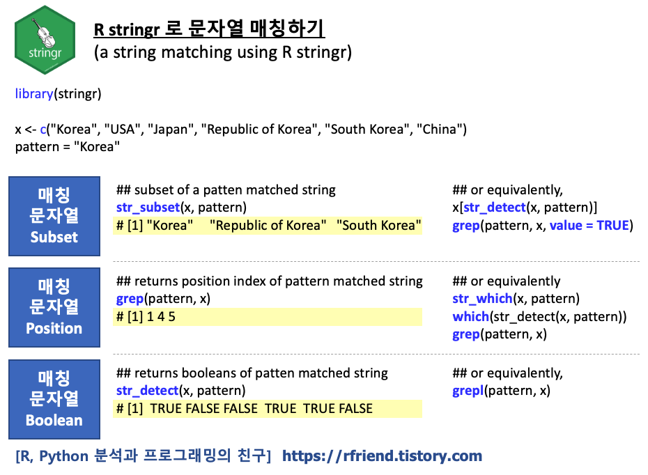
다음으로, "world" 의 'name_long' 칼럼의 원소 중에서 "Dem"으로 시작하고 "Congo"를 포함하고 있는 문자열을 stringr 패키지의 str_subset(string, pattern) 함수를 사용해 정규 표현식의 문자열 매칭으로 찾아보겠습니다. "world" 데이터셋의 'name_long' 칼럼에는 "Democratic Republic of the Congo" 라는 이름으로 데이터가 들어가 있네요. ("coffee_data" 데이터셋에는 "Confo, Dem. Rep. of" 라고 들어가 있다보니, 서로 같은 국가임에도 left_join() 을 했을 때 서로 정확하게 매칭이 안되어 Join 이 안되었습니다.)
참고로, str_subset() 은 x[str_detect(x, pattern)] 의 wrapper 입니다. 그리고 grep(pattern, x, value = TRUE) 와 동일한 역할을 수행합니다.
## setdiff(): calculates the set difference of subsets of two data frames
setdiff(coffee_data$name_long, world$name_long)
# [1] "Congo, Dem. Rep. of" "Others"


## string matching (regex) function from the stringr package
str_subset(world$name_long, "Dem*.+Congo")
# [1] "Democratic Republic of the Congo"
(3) 문자열 매칭으로 Key 값 업데이트 하고, 다시 두 테이블 inner join 하기
이제 Join Key로 사용하는 'name_long' 칼럼에서 "Congo" 국가에 대한 표기가 "world" 와 "coffee_data" 의 두 개 데이터셋이 서로 조금 다르다는 이유로 Join 이 안된다는 문제를 해결해 보겠습니다.
grepl(pattern, x) 함수로 "coffee_data" 데이터셋의 'name_long' 칼럼에서 "Congo" 가 들어있는 행을 찾아서, 그 행의 값의 str_subset() 의 정규표현식 문자열 매칭으로 찾은 (str_subset(world$name_long, "Dem*.+Congo") 이름인 "Demogratic Republic of the Congo" 라는 이름으로 대체를 해보겠습니다. 이렇게 하면 "world"와 "coffee_data"에 있는 "Congo" 국가의 긴 이름이 동일하게 "Demogratic Republic of Congo"로 되어 Join 이 제대로 될 것입니다.
## updating 'name_long' values using a string matching
coffee_data$name_long[grepl("Congo", coffee_data$name_long)] =
  str_subset(world$name_long, "Dem*.+Congo")

## inner join again using an updated key
world_coffee_match = inner_join(world, coffee_data)
#> Joining, by = "name_long"

nrow(world_coffee_match)
#> [1] 46
참고로, R에서 문자열 패턴 매칭을 할 때 grepl(pattern, x) 은 패턴 매칭되는 여부에 대해 TRUE, FALSE 로 블러언 값을 반환하는 반면에, grep(pattern, x) 은 패턴 매칭이 되는(TRUE) 위치 인덱스(Position Index)를 반환합니다.
## -- grepl: pattern matching and returns boolean
grepl("Congo", coffee_data$name_long)
# [1] FALSE FALSE FALSE FALSE FALSE FALSE  TRUE FALSE FALSE FALSE FALSE FALSE FALSE FALSE FALSE FALSE FALSE FALSE FALSE FALSE
# [21] FALSE FALSE FALSE FALSE FALSE FALSE FALSE FALSE FALSE FALSE FALSE FALSE FALSE FALSE FALSE FALSE FALSE FALSE FALSE FALSE
# [41] FALSE FALSE FALSE FALSE FALSE FALSE FALSE


## -- grep: pattern matching and returns position
grep("Congo", coffee_data$name_long)
# [1] 7
(4) Join 할 때 테이블 쓰는 순서의 중요성
dplyr 패키지로 두 테이블을 Join 할 때 왼쪽(x, LHS, Left Hand Side)에 써주는 테이블의 데이터 구조로 Join 한 결과를 반환합니다. 즉, Join 할 테이블을 써주는 순서가 중요합니다.
가령, 아래의 예에서는 "world" 가 'sf' 클래스의 지리 벡터 객체이고, 'coffee_data'는 tydiverse의 tibble, data.frame 객체입니다. left_join(world, coffee_data) 로 'world' 의 'sf' 지리 벡터 객체를 Join 할 때 왼쪽(LHS, x)에 먼저 써주면 Join 한 결과도 'sf' 클래스의 지리 벡터 객체가 됩니다.(R이 지리공간 벡터 데이터임을 알고 'sf' 클래스를 적용한 지리공간 데이터 처리 및 분석이 가능함).
반면에, left_join(coffee_data, world) 로 'coffee_data'의 'data.frame'을 Join 할 때 왼쪽(LHS, x)에 먼저 써주면 Join 한 결과도 'data.frame' 객체가 반환됩니다. (지리공간 'sf' 클래스가 더이상 아님)
## starting with a non-spatial dataset and
## adding variables from a simple features object.
## the result is not another simple feature object,
## but a data frame in the form of a tidyverse tibble:
## the output of a join tends to match its first argument.

## -- (a) 'sf' object first, then returns 'sf' object.
world_coffee = left_join(world, coffee_data)
#> Joining, by = "name_long"

class(world_coffee)
# [1] "sf"         "tbl_df"     "tbl"        "data.frame"


## -- (b) 'data.frame' object first, then returns 'data.frame' object.
coffee_world = left_join(coffee_data, world)
#> Joining, by = "name_long"

class(coffee_world)
#> [1] "tbl_df"     "tbl"        "data.frame"
(5) data.frame을 'sf' 클래스 객체로 변환하기
'sf' 패키지의 st_as_df() 함수를 사용하면 data.frame 을 'sf' 클래스 객체로 변환할 수 있습니다.
## -- converting data.frame to 'sf' class object

st_as_sf(coffee_world)

# imple feature collection with 47 features and 12 fields (with 2 geometries empty)
# geometry type:  MULTIPOLYGON
# dimension:      XY
# bbox:           xmin: -117.1278 ymin: -33.76838 xmax: 156.02 ymax: 35.49401
# geographic CRS: WGS 84
# # A tibble: 47 x 13
# name_long coffee_producti~ coffee_producti~ iso_a2 continent region_un subregion type  area_km2     pop lifeExp gdpPercap
# <chr>                <int>            <int> <chr>  <chr>     <chr>     <chr>     <chr>    <dbl>   <dbl>   <dbl>     <dbl>
#   1 "Angola"                NA               NA AO     Africa    Africa    Middle A~ Sove~ 1245464.  2.69e7    60.9     6257.
# 2 "Bolivia"                3                4 BO     South Am~ Americas  South Am~ Sove~ 1085270.  1.06e7    68.4     6325.
# 3 "Brazil"              3277             2786 BR     South Am~ Americas  South Am~ Sove~ 8508557.  2.04e8    75.0    15374.
# 4 "Burundi"               37               38 BI     Africa    Africa    Eastern ~ Sove~   26239.  9.89e6    56.7      803.
# 5 "Cameroo~                8                6 CM     Africa    Africa    Middle A~ Sove~  460325.  2.22e7    57.1     3196.
# 6 "Central~               NA               NA CF     Africa    Africa    Middle A~ Sove~  621860.  4.52e6    50.6      597.
# 7 "Congo, ~                4               12 NA     NA        NA        NA        NA         NA  NA         NA         NA
# 8 "Colombi~             1330             1169 CO     South Am~ Americas  South Am~ Sove~ 1151883.  4.78e7    74.0    12716.
# 9 "Costa R~               28               32 CR     North Am~ Americas  Central ~ Sove~   53832.  4.76e6    79.4    14372.
# 10 "C\u00f4~              114              130 CI     Africa    Africa    Western ~ Sove~  329826.  2.25e7    52.5     3055.
# # ... with 37 more rows, and 1 more variable: geom <MULTIPOLYGON [arc_degree]>
다음번 포스팅에서는 '지리공간 벡터 데이터에서 새로운 속성을 만들고 지리공간 정보를 제거하는 방법'에 대해서 알아보겠습니다.
[Reference]
- Geocomputation with R, 'Attribute data operations': geocompr.robinlovelace.net/attr.html
이번 포스팅이 많은 도움이 되었기를 바랍니다.
행복한 데이터 과학자 되세요! :-)