R, Python 분석과 프로그래밍의 친구 (by R Friend)

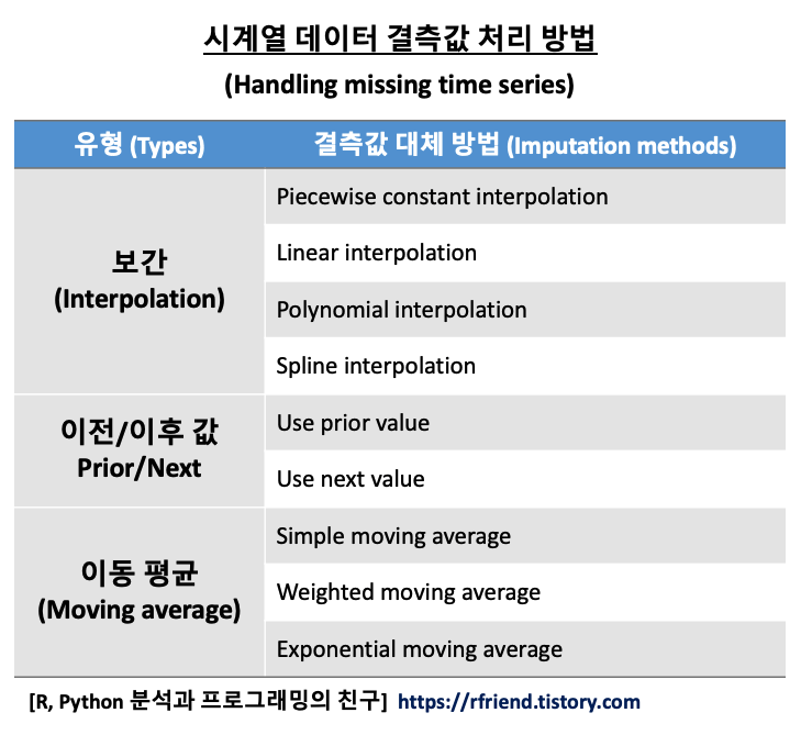
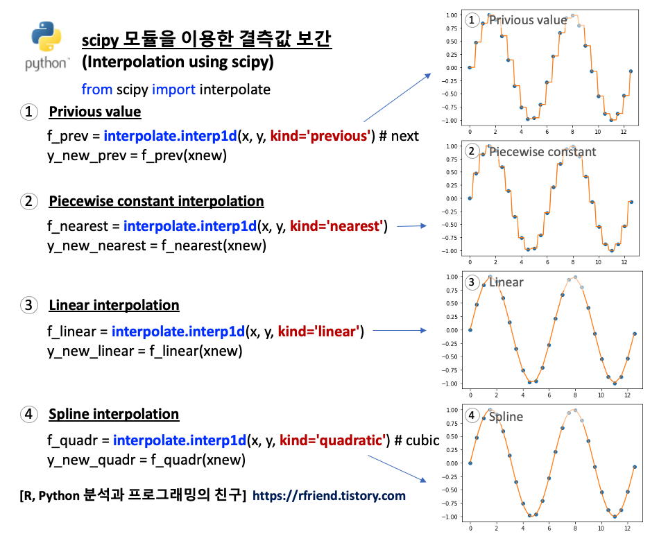
시계열 데이터를 분석할 때 제일 처음 확인하고 처리하는 일이 결측값(missing values) 입니다. 이번 포스팅에서는 시계열 데이터의 결측값을 선형 보간(linear interpolation)하는 2가지 방법을 소개하겠습니다. 

(1) Python 으로 결측값을 포함하는 예제 시계열 데이터 생성하기

(2) Python 의 for loop 순환문으로 시계열 데이터 결측값을 보간하기

      (interpolation sequentially using Python for loop statement)

(3) Greenplum에서 PL/Python으로 분산병렬처리하여 시계열 데이터 결측값을 보간하기

     (interpolation in parallel using PL/Python on Greenplum)

(1) Python 으로 결측값을 포함하는 예제 시계열 데이터 생성하기

샘플 시계열 데이터를 저장할 폴더를 base_dir 에 지정해주었습니다.

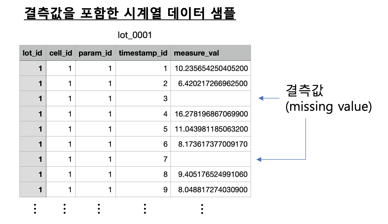
분석 단위로 사용할 Lot, Cell, Parameter, TimeStamp 의 개수를 지정해 줍니다. 아래 예에서는 각 Lot, Cell, Parameter 별로 100개의 TimeStamp 별로 측정값을 수집하고, 각 분석 단위별로 10개의 결측값을 포함하도록 설정했습니다. 

np.random.normal(10, 30, ts_num) 
: 측정값은 정규분포 X~N(10, 3) 의 분포로 부터 ts_num 인 100개를 난수 생성하여 만들었습니다. 

nan_mask = np.random.choice(np.arange(ts_num), missing_num)
ts_df_tmp.loc[nan_mask, 'measure_val'] = np.nan

: 각 분석 단위의 100 개의 측정치 중에서 무작위로 missing_num = 10 개를 뽑아서 np.nan 으로 교체하여 결측값으로 변경하였습니다.  

하나의 Lot에 Cell 100개, 각 Cell별 Parameter 10개, 각 Parameter 별 TimeStamp의 측정치 100개, 이중 결측치 10개를 포함한 시계열 데이터를 Lot 별로 묶어서(concat) DataFrame을 만들고, 이를 CSV 파일로 내보냅니다. 

#%% setting the directories and conditions
base_dir = '/Users/Documents/ts_data/'

## setting the number of IDs' conditions 
lot_num = 1000
cell_num = 100
param_num = 10
missing_num = 10
ts_num = 100 # number of TimeStamps


#%% [Step 1] generating the sample dataset

import numpy as np
import pandas as pd
import os
from itertools import chain, repeat

## defining the UDF
def ts_random_generator(lot_id, cell_num, param_num, ts_num, missing_num, base_dir):
    # blank DataFrame for saving the sample datasets later
    ts_df = pd.DataFrame()
    
    for cell_id in np.arange(cell_num):
        for param_id in np.arange(param_num):
            # making a DataFrame with colums of lot_id, cell_cd, param_id, ts_id, and measure_val
            ts_df_tmp = pd.DataFrame({
                'lot_id': list(chain.from_iterable(repeat([lot_id + 1], ts_num))), 
                'cell_id': list(chain.from_iterable(repeat([cell_id + 1], ts_num))), 
                'param_id': list(chain.from_iterable(repeat([param_id + 1], ts_num))), 
                'timestamp_id': (np.arange(ts_num) + 1), 
                'measure_val': np.random.normal(10, 3, ts_num)# X~N(mean, stddev, size)
            })
            
            # inserting the missing values randomly
            nan_mask = np.random.choice(np.arange(ts_num), missing_num)
            ts_df_tmp.loc[nan_mask, 'measure_val'] = np.nan
            
            # concatenate the generated random dataset(ts_df_tmp) to the lot based DataFrame(ts_df) 
            ts_df = pd.concat([ts_df, ts_df_tmp], axis=0)
    
    # exporting the DataFrame to local csv file
    base_dir = base_dir
    file_nm = 'lot_' + \
        str(lot_id+1).zfill(4) + \
        '.csv'
        
    ts_df.to_csv(os.path.join(base_dir, file_nm), index=False)
    #ts_df.to_csv('/Users/lhongdon/Documents/SK_ON_PoC/ts_data/lot_0001.csv')
    
    print(file_nm, "is successfully generated.") 



#%% Executing the ts_random_generator UDF above

## running the UDF above using for loop statement
for lot_id in np.arange(lot_num):
    ts_random_generator(
        lot_id, 
        cell_num, 
        param_num, 
        ts_num, 
        missing_num, 
        base_dir
        )

위의 코드를 실행하면 for loop 순환문이 lot_num 수만큼 돌면서 ts_random_generator() 사용자 정의함수를 실행시키면서 결측값을 포함한 시계열 데이터 샘플 CSV 파일을 생성하여 지정된 base_dir 폴더에 저장을 합니다. 

(아래 화면 캡쳐 참조)

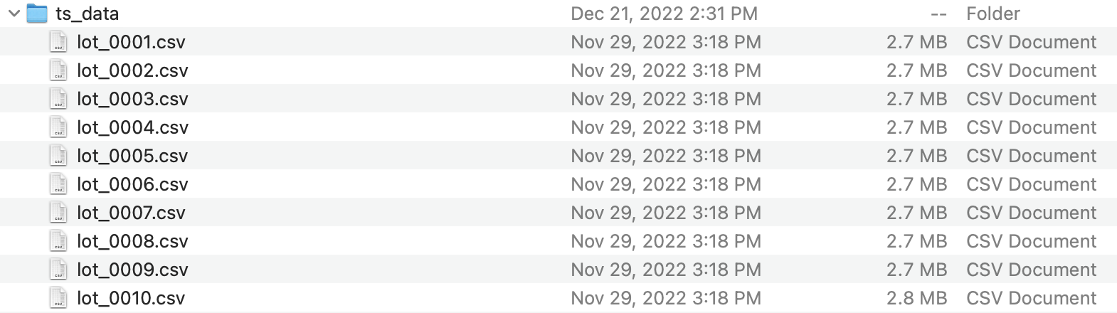
아래의 화면캡쳐는 결측값을 포함하는 시계열 데이터 샘플 중에서 LOT_0001 번의 예시입니다. 

(2) Python 의 for loop 순환문으로 시계열 데이터 결측값을 보간하기

      (interpolation sequentially using Python for loop statement)

아래 코드는 Python으로 Lot, Cell, Parameter ID 별로 for loop 순환문을 사용해서 pandas 의 interpolate() 메소드를 사용해서 시계열 데이터의 결측값을 선형 보간(linear interpolation) 한 것입니다. 

(forward fill 로 먼저 선형 보간을 해주고, 그 다음에 만약에 첫번째 행에 결측값이 있을 경우에 backward fill 로 이후 값과 같은 값으로 결측값을 채워줍니다.)

순차적으로 for loop 순환문을 돌기 때문에 시간이 오래 걸립니다.

#%% [Step 2] linear interpolation
from datetime import datetime
start_time = datetime.now()


## reading csv files in the base_dir
file_list = os.listdir(base_dir)

for file_nm in file_list:
    # by Lot
    if file_nm[-3:] == "csv":
        # read csv file
        ts_df = pd.read_csv(os.path.join(base_dir, file_nm))
        
        # blank DataFrame for saving the interpolated time series later
        ts_df_interpolated = pd.DataFrame()
        
        # cell & param ID lists
        cell_list = np.unique(ts_df['cell_id'])
        param_list = np.unique(ts_df['param_id'])
        
        # interpolation by lot, cell, and param IDs
        for cell_id in cell_list:
           for param_id in param_list:
               ts_df_tmp = ts_df[(ts_df.cell_id == cell_id) & (ts_df.param_id == param_id)]
               
               ## interpolating the missing values for equaly spaced time series data
               ts_df_tmp.sort_values(by='timestamp_id', ascending=True) # sorting by TimeStamp first
               ts_df_interpolated_tmp = ts_df_tmp.interpolate(method='values') # linear interploation
               ts_df_interpolated_tmp = ts_df_interpolated_tmp.fillna(method='bfill') # backward fill for the first missing row
               
               ts_df_interpolated = pd.concat([ts_df_interpolated, ts_df_interpolated_tmp], axis=0)
        
        # export DataFrame to local folder as a csv file
        ts_df_interpolated.to_csv(os.path.join(interpolated_dir, file_nm), index=False)
        
        print(file_nm, "is successfully interpolated.")


time_elapsed = datetime.now() - start_time
print("----------" * 5)
print("Time elapsed (hh:mm:ss.ms) {}".format(time_elapsed))
print("----------" * 5)

 

# # Before interplolation
# 3,1,1,20,11.160795506036791
# 3,1,1,21,8.155949904188175
# 3,1,1,22,3.1040644143505407
# 3,1,1,23,                   <-- missing
# 3,1,1,24,                   <-- missing
# 3,1,1,25,11.020504352275342
# 3,1,1,26,                   <-- missing
# 3,1,1,27,8.817922501760519
# 3,1,1,28,10.673174873272234
# 3,1,1,29,6.584669096660191
# 3,1,1,30,13.442427337943553

# # After interpolation
# 3,1,1,20,11.160795506036791
# 3,1,1,21,8.155949904188175
# 3,1,1,22,3.1040644143505407
# 3,1,1,23,5.742877726992141  <-- interpolated
# 3,1,1,24,8.381691039633742  <-- interpolated
# 3,1,1,25,11.020504352275342
# 3,1,1,26,9.919213427017931  <-- interpolated
# 3,1,1,27,8.81792250176052
# 3,1,1,28,10.673174873272234
# 3,1,1,29,6.584669096660191
# 3,1,1,30,13.442427337943554

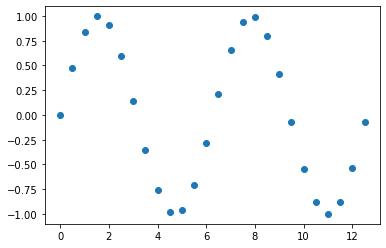
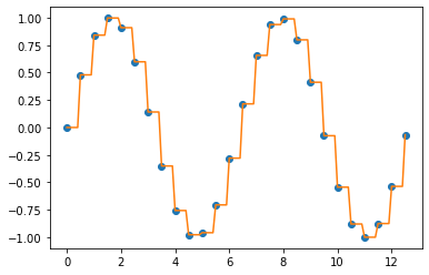
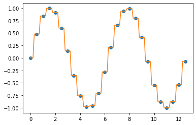
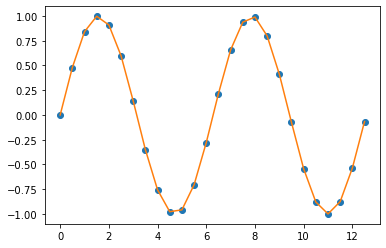
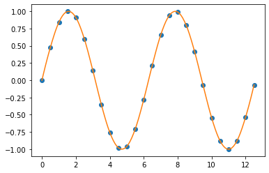
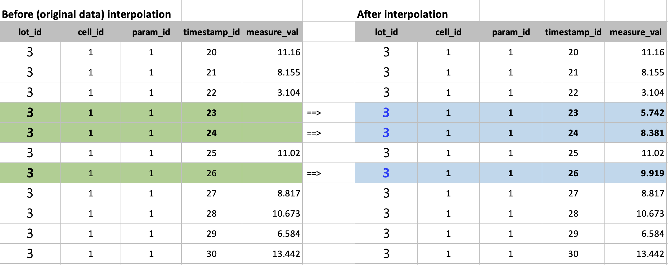
아래 화면캡쳐는 선형보간하기 전에 결측값이 있을 때와, 이를 선형보간으로 값을 생성한 후의 예시입니다. 

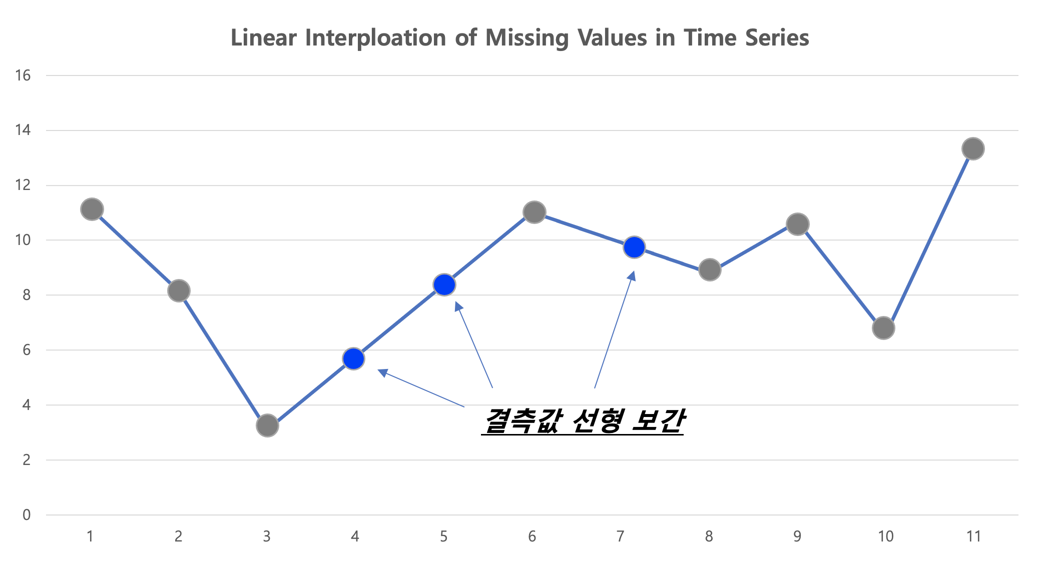
아래 선 그래프의 파란색 점 부분이 원래 값에서는 결측값 이었던 것을 선형 보간(linear interpolation)으로 채워준 후의 모습입니다. 선형보간이므로 측정된 값으로 선형회귀식을 적합하고, 결측값 부분의 X 값을 입력해서 Y를 예측하는 방식으로 결측값을 보간합니다. 

아래 코드는 데이터가 Greenplum DB에 적재되어 있다고 했을 때, 

 (2-1) Python으로 Greenplum DB에 access하여 데이터를 Query 해와서 pandas DataFrame으로 만들고 

 (2-2) Pytnon pandas 의 interpolate() 메소드를 사용해서 선형보간을 한 다음에 

 (2-3) 선형보간된 DataFrame을 pandas 의 to_sql() 메소드를 사용해서 다시 Greenplum DB에 적재

하는 코드입니다. 이를 for loop 순환문을 사용해서 Lot 의 개수만큼 실행시켜 주었습니다. 

순차적으로 for loop 순환문을 돌기 때문에 시간이 오래 걸립니다.

#%% Greenplum credentials
user = 'username' 
password = 'password' 
host = 'ip_address'
port = 'port'
db = 'databasename'

connection_string = "postgresql://{user}:{password}@{host}:{port}/{db}".\
        format(user=user, 
               password=password, 
               host=host, 
               port=port,
               db=db)

#%%
# helper function: query to pandas DataFrame
def gpdb_query(query):
    import psycopg2 as pg
    import pandas as pd
    
    conn = pg.connect(connection_string)
    cursor = conn.cursor()
    
    cursor.execute(query)
    col_names = [desc[0] for desc in cursor.description]
    
    result_df = pd.DataFrame(cursor.fetchall(), columns=col_names)
    
    cursor.close()
    conn.close()
    
    return result_df


#%% 
# UDF for running a query

def interpolator(lot_id):
    
    #import pandas as pd
    
    query = """
        SELECT * 
        FROM ts_data 
        WHERE 
            lot_id = {lot_id}
    """.format(
            lot_id = lot_id)
    
    ts_df = gpdb_query(query)
    ts_df = ts_df.astype({
        'measure_val': float
        })
    
    ## interpolating the missing values for equaly spaced time series data
    ts_df_interpolated = pd.DataFrame()
    
    for cell_id in (np.arange(cell_num)+1):
        for param_id in (np.arange(param_num)+1):
            ts_df_tmp = ts_df[(ts_df.cell_id == cell_id) & (ts_df.param_id == param_id)]
    
            ts_df_tmp.sort_values(by='timestamp_id', ascending=True) # sorting by TimeStamp first
            ts_df_interpolated_tmp = ts_df_tmp.interpolate(method='values') # linear interploation
            ts_df_interpolated_tmp = ts_df_interpolated_tmp.fillna(method='bfill') # backward fill for the first missing row
            
            ts_df_interpolated = pd.concat([ts_df_interpolated, ts_df_interpolated_tmp], axis=0)
    
    # export DataFrame to local folder as a csv file
    #ts_df_interpolated.to_csv(os.path.join(interpolated_dir, file_nm), index=False)        
    #print(file_nm, "is successfully interpolated.")
    
    return ts_df_interpolated



#%% 
# UDF for importing pandas DataFrame to Greenplum DB
def gpdb_importer(lot_id, connection_string):
    
    import sqlalchemy
    from sqlalchemy import create_engine
    
    engine = create_engine(connection_string)
    
    # interpolation
    ts_data_interpolated = interpolator(lot_id)
    
    # inserting to Greenplum    
    ts_data_interpolated.to_sql(
        name = 'ts_data_interpolated_python', 
        con = engine, 
        schema = 'equipment', 
        if_exists = 'append', 
        index = False, 
        dtype = {'lot_id': sqlalchemy.types.INTEGER(), 
                 'cell_id': sqlalchemy.types.INTEGER(), 
                 'param_id': sqlalchemy.types.INTEGER(),
                 'timestamp_id': sqlalchemy.types.INTEGER(), 
                 'measure_val': sqlalchemy.types.Float(precision=6)
                 })
    

#%%
from datetime import datetime
start_time = datetime.now()

import pandas as pd
import os
import numpy as np

for lot_id in (np.arange(lot_num)+1):
    gpdb_importer(lot_id, connection_string)
    print("lot_id", lot_id, "is successfully interpolated.")

time_elapsed = datetime.now() - start_time
print("----------" * 5)
print("Time elapsed (hh:mm:ss.ms) {}".format(time_elapsed))
print("----------" * 5)

(3) Greenplum에서 PL/Python으로 분산병렬처리하여 시계열 데이터 결측값을 보간하기

     (interpolation in parallel using PL/Python on Greenplum)

Greenplum에서 PL/Python으로 병렬처리할 때는 (a) 사용자 정의 함수(UDF) 정의, (b) 사용자 정의 함수 실행의 두 단계를 거칩니다. 

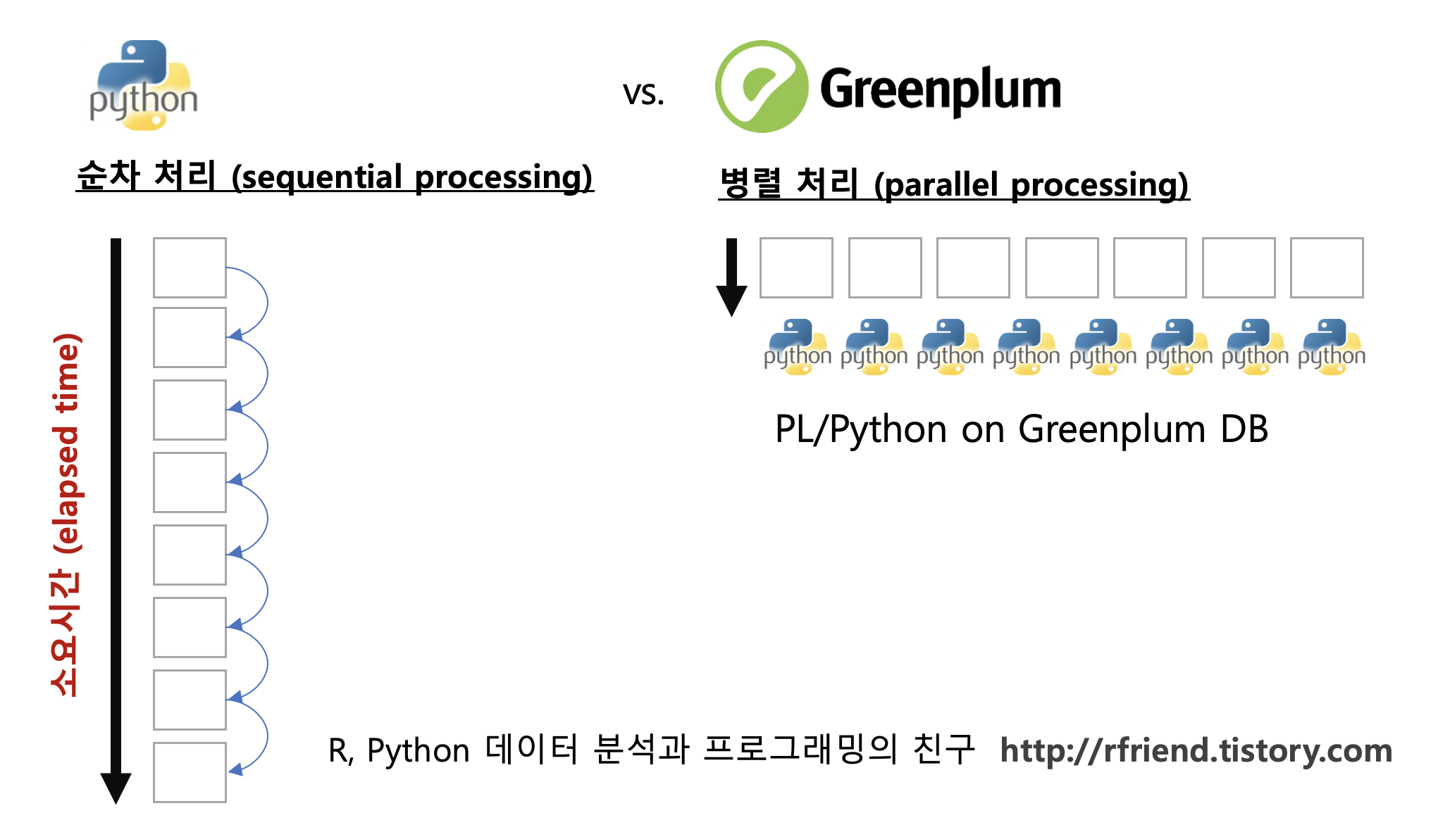
Greenplum DB에서 PL/Python으로 분산병렬처리를 하면 위의 (2)번에서 Python으로 for loop 순환문으로 순차처리한 것 대비 Greenplum DB 내 노드의 개수에 비례하여 처리 속도가 줄어들게 됩니다. (가령, 노드가 8개이면 병렬처리의 총 처리 소요시간은 순차처리했을 때의 총 소요시간의 1/8 로 줄어듭니다.) 

(3-1) PL/Python 으로 시계열 데이터 결측값을 선형보간하는 사용자 정의함수 정의 (define a UDF)

-- defining the PL/Python UDF
DROP FUNCTION IF EXISTS plpy_interp(numeric[]);
CREATE OR REPLACE FUNCTION plpy_interp(measure_val_arr numeric[]) 
RETURNS numeric[]
AS $$
	import numpy as np
	import pandas as pd
	
	measure_val = np.array(measure_val_arr, dtype='float')
	
	ts_df = pd.DataFrame({
	   'measure_val': measure_val
	    })
	
	# interpolation by lot, cell, and param IDs               
	ts_df_interpolated = ts_df.interpolate(method='values') # linear interploation
	ts_df_interpolated = ts_df_interpolated.fillna(method='bfill') # backward fill for the first missing row
	
	return ts_df_interpolated['measure_val']
	        
$$ LANGUAGE 'plpythonu';

(3-2) 위에서 정의한 시계열 데이터 결측값을 선형보간하는 PL/Python 사용자 정의함수 실행

PL/Python의 input 으로는 SQL의 array_agg() 함수를 사용해서 만든 Array 데이터를 사용하며, PL/Python에서는 SQL의 Array를 Python의 List 로 변환(converting) 합니다. 

-- array aggregation as an input
DROP TABLE IF EXISTS tab1;
CREATE TEMPORARY TABLE tab1 AS
		SELECT 
			lot_id
			, cell_id
			, param_id
			, ARRAY_AGG(timestamp_id ORDER BY timestamp_id) AS timestamp_id_arr
			, ARRAY_AGG(measure_val ORDER BY timestamp_id) AS measure_val_arr
		FROM ts_data
		GROUP BY lot_id, cell_id, param_id
DISTRIBUTED RANDOMLY ;
		
ANALYZE tab1;		


-- executing the PL/Python UDF
DROP TABLE IF EXISTS ts_data_interpolated;
CREATE TABLE ts_data_interpolated AS (
	SELECT 
		lot_id 
		, cell_id 
		, param_id 
		, timestamp_id_arr
		, plpy_interp(measure_val_arr) AS measure_val_arr -- plpython UDF
	FROM tab1 AS a 
) DISTRIBUTED BY (lot_id);

아래 코드는 numeric array 형태로 반환한 선형보간 후의 데이터를 unnest() 함수를 사용해서 보기에 편하도록 long format 으로 풀어준 것입니다. 

-- display the interpolated result
SELECT 
	lot_id
	, cell_id 
	, param_id
	, UNNEST(timestamp_id_arr) AS timestamp_id
	, UNNEST(measure_val_arr) AS measure_val
FROM ts_data_interpolated
WHERE lot_id = 1 AND cell_id = 1 AND param_id = 1
ORDER BY lot_id, cell_id, param_id, timestamp_id
LIMIT 100;

결측값을 포함하고 있는 원래 데이터셋을 아래 SQL query 로 조회해서, 위의 선형보간 된 후의 데이터셋과 비교해볼 수 있습니다. 

-- original dataset with missing value
SELECT 
	lot_id
	, cell_id 
	, param_id
	, timestamp_id
	, measure_val
FROM ts_data
WHERE lot_id = 1 AND cell_id = 1 AND param_id = 1
ORDER BY lot_id, cell_id, param_id, timestamp_id
LIMIT 100;

이번 포스팅이 많은 도움이 되었기를 바랍니다. 

행복한 데이터 과학자 되세요!  :-)

시계열 데이터를 분석할 때 꼭 확인하고 처리해야 하게 있는데요, 바로 결측값 여부 확인과 결측값 처리입니다. 

시계열 데이터의 결측값을 처리하는 방법에는

   (1) 보간 (Interpolation)

   (2) 이전 값 또는 다음 값 이용 (previous/next value)

   (3) 이동 평균 (Moving average)

등의 여러가지 방법이 있습니다. 

[ 시계열 데이터 결측값 처리 방법 (How to handle the time series missing data) ]

아래의 보간(Interpolation)에 대한 내용은 Wikipedia 의 내용을 번역하여 소개합니다. 

데이터 분석의 수학 분야에서는 "보간법(Interpolation)을 이미 알려진 데이터 포인트들의 이산형 집합의 범위에 기반해서 새로운 데이터 포인트들을 만들거나 찾는 추정(estimation)의 한 유형"으로 봅니다. 

공학과 과학 분야에서는 종종 샘플링이나 실험을 통해서 많은 수의 데이터 포인트들을 획득하는데요, 이들 데이터는 어떤 함수(a function)의 값이나 독립변수(independent variable)의 제한적인 수의 값을 표현한 것입니다. 종종 독립변수의 중간 사이의 값을 위한 함수의 값을 추정(estimate the value of that function for an intermediat value of the independent variable)하는 보간이 필요합니다.  

밀접하게 관련된 문제로서 복잡한 함수를 간단한 함수로 근사하게 추정(the approximation of a complicated function by a simple function)하는 것이 있습니다. 어떤 주어진 함수의 공식이 알려져있지만, 너무 복잡해서 효율적으로 평가하기가 어렵다고 가정해봅시다. 원래의 함수로부터 적은 수의 새로운 데이터 포인트는 원래의 값과 상당히 근접한 간단한 함수를 생성해서 보간할 수 있습니다. 단순성(simplicity)으로부터 얻을 수 있는 이득이 보간에 의한 오차라는 손실보다 크고, 연산 프로세스면서도 더 좋은 성능(better performance in calculation process)을 낼 수도 있습니다.   

이번 포스팅에서는 Python scipy 모듈을 이용해서 시계열 데이터 결측값을 보간(Interpolation)하는 방법을 소개하겠습니다. 

1. 이전 값/ 이후 값을 이용하여 결측값 채우기 (Imputation using the previous/next values)

2. Piecewise Constant Interpolation

3. 선형 보간법 (Linear Interpolation)

4. 스플라인 보간법 (Spline Interpolation)

[ Python scipy 모듈을 이용한 결측값 보간 (Interpolation using Python scipy module)  ]

먼저 '0.5'로 동일한 간격을 가지는 x 값들에 대한 사인 함수 (sine function) 의 y값을 계산해서  예제 데이터로 사용하겠습니다. 아래 예졔의 점과 점 사이의 값들이 비어있는 결측값이라고 간주하고, 이들 값을 채워보겠습니다. 

import numpy as np
from scipy import interpolate
import matplotlib.pyplot as plt

## generating the original data with missing values
x = np.arange(0, 4*np.pi, 0.5)
y = np.sin(x)

plt.plot(x, y, "o")
plt.show()

1. 이전 값/ 다음 값을 이용하여 결측값 채우기 (Imputation using the previous/next values)

데이터 포인트 사이의 값을 채우는 가장 간단한 방법은 이전 값(previous value) 나 또는 다음 값(next value)을 이용하는 것입니다. 함수를 추정하는 절차가 필요없으므로 연산 상 부담이 적지만, 데이터 추정 오차는 단점이 될 수 있습니다. 

## Interpolation using the previous value
f_prev = interpolate.interp1d(
    x, y, kind='previous') # next
y_new_prev = f_prev(xnew)

plt.plot(x, y, "o", xnew, y_new_prev, '-')
plt.show()

2. Piecewise Constant Interpolation

위 1번의 이전 값 또는 다음 값을 이용한 사이값 채우기를 합쳐놓은 방법입니다. Piecewise Constant Interpolation은 특정 데이터 포인트를 기준으로 가장 가까운 값 (nearest value) 을 가져다가 사이값을 보간합니다. ("최근접 이웃 보간"이라고도 함)

간단한 문제에서는 아래 3번에서 소개하는 Linear Interpolation 이 주로 사용되고, Piecewise Constant Interpolation 은 잘 사용되지 않는 편입니다. 하지만 다차원의 다변량 보간 (in higher-dimensional multivariate interpolation)의 경우, 속도와 단순성(speed and simplicity) 측면에서 선호하는 선택이 될 수 있습니다. 

## Piecewise Constant Interpolation
f_nearest = interpolate.interp1d(
    x, y, kind='nearest')

y_new_nearest = f_nearest(xnew)

plt.plot(x, y, "o", xnew, y_new_nearest)
plt.show()

3. Linear Interpolation

선형 보간법은 가장 쉬운 보간법 중의 하나로서, 연산이 빠르고 쉽습니다. 하지만 추정값이 정확한 편은 아니며, 데이터 포인트 Xk 에서 미분 가능하지 않다는 단점도 있습니다. 

일반적으로, 선형 보간법은 두 개의 데이터 포인트, 가령 (Xa, Ya)와 (Xb, Yb), 를 사용해서 다음의 공식으로 두 값 사이의 값을 보간합니다. 

Y = Ya + (Yb - Ya) * (X - Xa) / (Xb- Xa)    at the point (x, y)

## Linear Interpolation
f_linear = interpolate.interp1d(
    x, y, kind='linear')

y_new_linear = f_linear(xnew)

plt.plot(x, y, "o", xnew, y_new_linear, '-')
plt.show()

4. Spline Interpolation

다항식 보간법(Polynomial Interpolation)은 선형 보간법을 일반화(generalization of linear interpolation)한 것입니다. 선형 보간법에서는 선형 함수를 사용했다면, 다항식 보간법에서는 더 높은 차수의 다항식 함수를 사용해서 보간하는 것으로 대체한 것입니다. 

일반적으로, 만약 우리가 n개의 데이터 포인트를 가지고 있다면 모든 데이터 포인트를 통과하는 n-1 차수의 다차항 함수가 존재합니다. 보간 오차는 데이터 포인트 간의 거리의 n 차승에 비례(interpolation error is proportional to the distance between the data points to the power n)하며, 다차항 함수는 미분가능합니다. 따라서 선형 보간법의 대부분의 문제를 다항식 보간법은 극복합니다. 하지만 다항식 보간법은 선형 보간법에 비해 복잡하고 연산에 많은 비용이 소요됩니다. 그리고 끝 점(end point) 에서는 진동하면서 변동성이 큰 값을 추정하는 문제가 있습니다. 

스플라인 보간법은 각 데이터 포인트 구간별로 낮은 수준의 다항식 보간을 사용 (Spline interpolation uses low-degree polynomials in each of the intervals) 합니다. 그리고 이들이 함께 부드럽게 연결되어서 적합될 수 있도록 다항식 항목을 선택(, and chooses the polynomial pieces such that they fit smoothly together)합니다. 이렇게 적합된 함수를 스플라인(Spline) 이라고 합니다. 

스플라인 보간법(Spline Interpolation)은 다항식 보간법의 장점은 살리고 단점은 피해간 보간법입니다. 스플라인 보간법은 다항식 보간법처럼 선형 보간법보다 보간 오차가 더 작은 반면에, 고차항의 다항식 보간법보다는 보간 함수가 부드럽고 평가하기가 쉽습니다.  

## Spline Interpolation
f_quadr = interpolate.interp1d(
    x, y, kind='quadratic') # cubic

y_new_quadr = f_quadr(xnew)

plt.plot(x, y, "o", xnew, y_new_quadr)
plt.show()

[ Reference ]

1. 보간법(interpolation): https://en.wikipedia.org/wiki/Interpolation

2. scipy 모듈: https://docs.scipy.org/doc/scipy/reference/generated/scipy.interpolate.interp1d.html

이번 포스팅이 많은 도움이 되었기를 바랍니다.

행복한 데이터 과학자 되세요!  :-)

지난번 포스팅에서는 Python pandas에서 resampling 중 Downsampling 으로 집계할 때에 왼쪽과 오른쪽 중에서 어느쪽을 포함(inclusive, closed)할 지와 어느쪽으로 라벨 이름(label)을 쓸지(https://rfriend.tistory.com/507)에 대해서 알아보았습니다. 

이번 포스팅에서는 pandas의 resampling 중 Upsampling으로 시계열 데이터 주기(frequency)를 변환(conversion) 할 때 생기는 결측값을 처리하는 두 가지 방법을 소개하겠습니다. 

(1) Upsampling 으로 주기 변환 시 생기는 결측값을 채우는 방법 (filling forward/backward)

(2) Upsampling 으로 주기 변환 시 생기는 결측값을 선형 보간하는 방법 (linear interpolation)

예제로 사용할 간단할 2개의 칼럼을 가지고 주기(frequency)가 5초(5 seconds)인 시계열 데이터 DataFrame을 만들어보겠습니다. 

[Out]:
DatetimeIndex(['2019-12-31 00:00:00', '2019-12-31 00:00:05',
               '2019-12-31 00:00:10'],
              dtype='datetime64[ns]', freq='5S')

이제 pandas resample() 메소드를 사용해서 주기가 5초(freq='5S')인 원래 데이터를 주기가 1초(freq='1S')인 데이터로 Upsampling 변환을 해보겠습니다. 그러면 아래처럼 새로 생긴 날짜-시간 행에 결측값(missing value)이 생깁니다ㅣ  

위에 Upsampling을 해서 생긴 결측값들을 (1) 채우기(filling), (2) 선형 보간(linear interpolation) 해보겠습니다. 

(1-1) 앞의 값으로 뒤의 결측값 채우기 (Filling forward)

(1-2) 뒤의 값으로 앞의 결측값 채우기 (Filling backward)

(1-3) 특정 값으로 결측값 채우기

(1-4) 평균 값으로 결측값 채우기

[Out]:

col_1    4.333333
col_2    2.000000
dtype: float64

(1-5) 결측값 채우는 행의 개수 제한하기

많은 도움이 되었기를 바랍니다. 

이번 포스팅이 도움이 되었다면 아래의 '공감~'를 꾹 눌러주세요. :-)