[R] R Shiny로 두 연속형 변수 간 상관계수, 산점도와 회귀선 그리는 앱 애플리케이션 만들기
R 분석과 프로그래밍/R 동적 문서(Dynamic Document) 2019. 6. 30. 22:07이번 포스팅에서는 R Shiny를 사용하여 interactive하게 편하고 쉽게 두 연속형 변수 간 관계를 알아볼 수 있도록
(1) 상관계수 (Correlation Coefficient)를 구하고,
(2) 산점도 (Scatter Plot)을 그린 후,
(3) 선형 회귀선 (Linear Regression Line) 을 겹쳐서 그려주는
웹 애플리케이션을 만들어보겠습니다.
예제로 사용할 데이터는 MASS 패키지에 내장되어 있는 Cars93 데이터프레임으로서, Price, MPG.city, MPG.highway, EngineSize, Horsepower, RPM 의 6개 연속형 변수를 선별하였습니다.
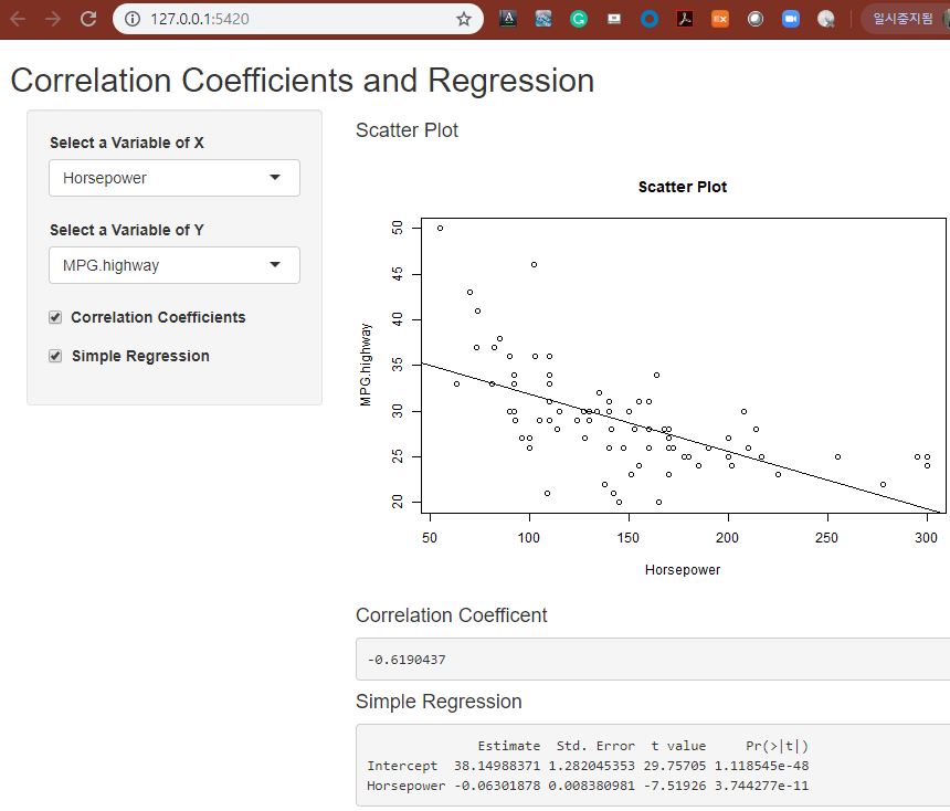
왼쪽 사이드바 패널에는 산점도의 X축, Y축에 해당하는 연속형 변수를 콤보박스로 선택할 수 있도록 하였으며, 상관계수와 선형회귀모형을 적합할 지 여부를 선택할 수 있는 체크박스도 추가하였습니다.
오른쪽 본문의 메인 패널에는 두 연속형 변수에 대한 산점도 그래프에 선형 회귀선을 겹쳐서 그려서 보여주고, 상관계수와 선형회귀 적합 결과를 텍스트로 볼 수 있도록 화면을 구성하였습니다.
|
library(shiny) # Define UI for application that analyze correlation coefficients and regression ui <- fluidPage(
# Application title titlePanel("Correlation Coefficients and Regression"),
# Select 2 Variables, X and Y sidebarPanel( selectInput("var_x", label = "Select a Variable of X", choices = list("Price"="Price", "MPG.city"="MPG.city", "MPG.highway"="MPG.highway", "EngineSize"="EngineSize", "Horsepower"="Horsepower", "RPM"="RPM"), selected = "RPM"),
selectInput("var_y", label = "Select a Variable of Y", choices = list("Price"="Price", "MPG.city"="MPG.city", "MPG.highway"="MPG.highway", "EngineSize"="EngineSize", "Horsepower"="Horsepower", "RPM"="RPM"), selected = "MPG.highway"),
checkboxInput(inputId = "corr_checked", label = strong("Correlation Coefficients"), value = TRUE),
checkboxInput(inputId = "reg_checked", label = strong("Simple Regression"), value = TRUE) ), # Show a plot of the generated distribution mainPanel( h4("Scatter Plot"), plotOutput("scatterPlot"),
h4("Correlation Coefficent"), verbatimTextOutput("corr_coef"),
h4("Simple Regression"), verbatimTextOutput("reg_fit") ) ) # Define server logic required to analyze correlation coefficients and regression server <- function(input, output) { library(MASS) scatter <- Cars93[,c("Price", "MPG.city", "MPG.highway", "EngineSize", "Horsepower", "RPM")]
# scatter plot output$scatterPlot <- renderPlot({ var_name_x <- as.character(input$var_x) var_name_y <- as.character(input$var_y)
plot(scatter[, input$var_x], scatter[, input$var_y], xlab = var_name_x, ylab = var_name_y, main = "Scatter Plot")
# add linear regression line fit <- lm(scatter[, input$var_y] ~ scatter[, input$var_x]) abline(fit) })
# correlation coefficient output$corr_coef <- renderText({ if(input$corr_checked){ cor(scatter[, input$var_x], scatter[, input$var_y]) } })
# simple regression output$reg_fit <- renderPrint({ if(input$reg_checked){ fit <- lm(scatter[, input$var_y] ~ scatter[, input$var_x]) names(fit$coefficients) <- c("Intercept", input$var_x) summary(fit)$coefficients } }) } # Run the application shinyApp(ui = ui, server = server) |
많은 도움이 되었기를 바랍니다.

'R 분석과 프로그래밍 > R 동적 문서(Dynamic Document)' 카테고리의 다른 글
| [R] R Shiny 로 두 집단 간 평균 차이 t-검정(t-Test) 신뢰수준별 신뢰구간 구하는 웹 애플리케이션 만들기 (5) | 2019.06.30 |
|---|---|
| [R] R Shiny로 연속형 변수 별 요약 통계량 조회하는 Interactive App 만들기 (0) | 2019.06.29 |
| [R] rmarkdown HTML 문서의 포맷 정하기 (7) | 2017.05.02 |
| [R] servr 패키지를 사용해서 .Rmd 파일들을 자동 rendering 하고 로컬 웹 서버로 올리기 (0) | 2017.05.01 |
| [R] RStudio 를 사용해서 HTML 문서 만들기 (2) | 2017.04.30 |


