[Python] 통계적 가설 검정을 통한 시계열 정상성 여부 확인 (checking stationarity using statistical hypothesis test: ADF test, KPSS test)
Python 분석과 프로그래밍/Python 통계분석 2021. 10. 10. 23:55지난번 포스팅에서는 백색잡음과정(White noise process), 확률보행과정(Random walk process), 정상확률과정(Stationary process)에 대해서 소개하였습니다. (https://rfriend.tistory.com/691)
지난번 포스팅에서 특히 ARIMA와 같은 시계열 통계 분석 모형이 정상확률과정(Stationary Process)을 가정한다고 했습니다. 따라서 시계열 통계 모형을 적합하기 전에 분석 대상이 되는 시계열이 정상성 가정(Stationarity assumption)을 만족하는지 확인을 해야 합니다.
[ 정상확률과정 (stationary process) 정의 ]
1. 평균이 일정하다.
2. 분산이 존재하며, 상수이다.
3. 두 시점 사이의 자기공분산은 시차(時差, time lag)에만 의존한다.
정상 시계열 (stationary time series) 여부를 확인하는 방법에는 3가지가 있습니다.
[1] 시계열 그래프 (time series plot)
[2] 통계적 가설 검정 (statistical hypothesis test)
[3] 자기상관함수(ACF), 편자기상관함수(PACF)
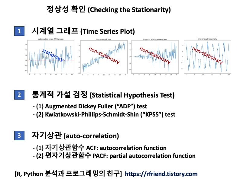
이번 포스팅에서는 이중에서 통계적 가설 검정 (Statistical Hypothesis Test) 을 이용해 정상성(stationarity) 여부를 확인하는 방법을 소개하겠습니다.
- (a) Augmented Dickey-Fuller (“ADF”) test
- (b) Kwiatkowski-Phillips-Schmidt-Shin (“KPSS”) test
ADF 검정은 시계열에 단위근(unit root)이 존재하는지의 여부를 검정함으로써 정상 시계열인지 여부를 판단합니다. 단위근이 존재하면 정상 시계열이 아닙니다.
단위근(unit root)이란 확률론의 데이터 검정에서 쓰이는 개념입니다. 주로 ‘단위근 검정’의 형식으로 등장합니다. 일반적으로 시계열 데이터는 시간에 따라 일정한 규칙을 가짐을 가정합니다. 따라서 매우 복잡한 형태를 갖는 시계열 데이터라도 다음과 같은 식으로 어떻게든 단순화시킬 수 있을 것이라 생각해볼 수 있습니다.

즉, ‘t시점의 확률변수는 t-1, t-2 시점의 확률변수와 관계를 가지면서 거기에 에러가 포함된 것’이라는 의미입니다. 여기서 편의를 위해 y0=0이라 가정합니다. 이제 아래의 방정식을 볼까요.

여기서 m=1이 위 식의 근이 된다면 이때의 시계열 과정을 단위근을 가진다고 합니다. 단위근 모형은 주로 복잡한 시계열 데이터를 단순하게나마 계산하려 할 때 사용됩니다.
Python으로 가상의 시계열 데이터셋(1개의 정상 시계열, 3개의 비정상 시계열)을 만들어서 위의 ADF test, KPSS test 를 각각 해보겠습니다. 위의 정상확률과정의 정의에 따라서, 추세(trend)가 있거나, 분산(variance)이 시간의 흐름에 따라 변하거나(증가 또는 감소), 계절성(seasonality)을 가지고 있는 시계열은 정상성(stationarity) 가정을 만족하지 않습니다.
- (1) 정상 시계열 데이터 (stationary time series)
- (2) 추세를 가진 비정상 시계열 데이터 (non-stationary time series with trend)
- (3) 분산이 변하는 비정상 시계열 데이터 (non-stationary time series with changing variance)
- (4) 계절성을 가지는 비정상 시계열 데이터 (non-stationary time series with seasonality)
이제 (1)~(4)번 데이터별로 (a) ADF test, (b) KPSS test 로 정상성 여부를 차례대로 가설 검정해보겠습니다.
(1) 정상 시계열 데이터 (stationary time series)
먼저, 자기회귀과정(auto-regressive process)을 따르는 AR(1) 과정의 시계열 데이터를 임의로 만들어보겠습니다.
import numpy as np
import matplotlib.pyplot as plt

## Stationary Process
## exmaple: AR(1) process
np.random.seed(1) # for reproducibility
z_0 = 0
rho = 0.6 # correlation b/w z(t) and z(t-1)
z_all = [z_0]

for i in range(200):
    z_t = rho*z_all[i] + np.random.normal(0, 0.1, 1)
    z_all.append(z_t)

## plotting
plt.rcParams['figure.figsize'] = (10, 6)
plt.plot(z_all)
plt.title("stationary time series : AR(1) process", fontsize=16)

## adding horizonal line at mean position 0
plt.axhline(0, 0, 200, color='red', linestyle='--', linewidth=2)
plt.show()
(1-a) ADF 검정 (Augmented Dickey-Fuller test)
Python의 statsmodels 모듈에 있는 adfuller 메소드를 사용해서 ADF 검정을 위한 사용자 정의함수를 정의해보겠습니다.
#! pip install statsmodels

## UDF for ADF test
from statsmodels.tsa.stattools import adfuller
import pandas as pd

def adf_test(timeseries):
    print("Results of Dickey-Fuller Test:")
    dftest = adfuller(timeseries, autolag="AIC")
    dfoutput = pd.Series(
        dftest[0:4],
        index=[
            "Test Statistic",
            "p-value",
            "#Lags Used",
            "Number of Observations Used",
        ],
    )
    for key, value in dftest[4].items():
        dfoutput["Critical Value (%s)" % key] = value
    print(dfoutput)
이제 위에서 만든 ADF 검정 사용자정의함수 adf_test() 를 사용해서 정상시계열 z_all 에 대해서 ADF 검정을 해보겠습니다. p-value 가 8.74e-11 이므로 유의수준 5% 하에서 귀무가설 (H0: 단위근(unit root)이 존재한다. 즉, 정상 시계열이 아니다)을 기각하고 대립가설 (H1: 단위근이 없다. 즉, 정상 시계열이다.) 을 채택합니다. (맞음 ^_^)
## checking the stationarity of a series using the ADF(Augmented Dickey-Fuller) Test
# -- Null Hypothesis: The series has a unit root.(not stationary.)
# -- Alternate Hypothesis: The series has no unit root.(stationary.)

adf_test(z_all)  # p-value 8.740428e-11 => stationary

# Results of Dickey-Fuller Test:
# Test Statistic                -7.375580e+00
# p-value                        8.740428e-11
# #Lags Used                     1.000000e+00
# Number of Observations Used    1.990000e+02
# Critical Value (1%)           -3.463645e+00
# Critical Value (5%)           -2.876176e+00
# Critical Value (10%)          -2.574572e+00
# dtype: float64
이번에는 Python의 statsmodels 모듈을 사용해서 KPSS 검정 (Kwiatowski-Phillips-Schmidt-Shin Test) 을 위한 사용자 정의함수를 정의해보겠습니다.
## UDF for KPSS test
from statsmodels.tsa.stattools import kpss
import pandas as pd

def kpss_test(timeseries):
    print("Results of KPSS Test:")
    kpsstest = kpss(timeseries, regression="c", nlags="auto")
    kpss_output = pd.Series(
        kpsstest[0:3], index=["Test Statistic", "p-value", "Lags Used"]
    )
    for key, value in kpsstest[3].items():
        kpss_output["Critical Value (%s)" % key] = value
    print(kpss_output)
이제 정상 시계열 z_all 에 대해서 위에서 정의한 kpss_test() 함수를 사용해서 정상성 여부를 확인해보겠습니다. p-value 가 0.065 로서 유의수준 10% 하에서 귀무가설 (H0: 정상 시계열이다) 를 채택하고, 대립가설 (H1: 정상 시계열이 아니다) 를 기각합니다. (유의수준 5% 하에서는 대립가설 채택). (맞음 ^_^)
* 이때, KPSS 검정은 ADF 검정과는 귀무가설과 대립가설이 정반대이므로 해석에 조심하시기 바랍니다.
kpss_test(z_all) # p-value 0.065035 => stationary at significance level 10%

# Results of KPSS Test:
# Test Statistic           0.428118
# p-value                  0.065035
# Lags Used                5.000000
# Critical Value (10%)     0.347000
# Critical Value (5%)      0.463000
# Critical Value (2.5%)    0.574000
# Critical Value (1%)      0.739000
# dtype: float64
(2) 추세를 가진 비정상 시계열 데이터 (non-stationary time series with trend)
다음으로, 추세(trend)를 가지는 가상의 비정상(non-stationary) 시계열 데이터를 만들어보겠습니다. 평균이 일정하지 않으므로 비정상 시계열이 되겠습니다.
## time series with trend
np.random.seed(1) # for reproducibility
ts_trend = 0.01*np.arange(200) + np.random.normal(0, 0.2, 200)

## plotting
plt.plot(ts_trend)
plt.title("time series with trend", fontsize=16)

plt.show()
(2-a) ADF 검정 (ADF test)
위의 추세를 가지는 비정상 시계열 데이터에 대해 ADF 검정 (ADF test)를 실시해보면, p-value가 0.96 으로서 유의수준 5% 하에서 귀무가설 (H0: 시계열이 단위근을 가진다. 즉, 정상 시계열이 아니다) 을 채택하고, 귀무가설 (H1: 시계열이 단위근을 가지지 않는다. 즉, 정상 시계열이다.) 을 기각합니다. (맞음 ^_^)
## checking the stationarity of a series using the ADF(Augmented Dickey-Fuller) Test
# -- Null Hypothesis: The series has a unit root.(not stationary.)
# -- Alternate Hypothesis: The series has no unit root.(stationary.)

adf_test(ts_trend) # p-value 0.96 => non-stationary

# Results of Dickey-Fuller Test:
# Test Statistic                   0.125812
# p-value                          0.967780
# #Lags Used                      10.000000
# Number of Observations Used    189.000000
# Critical Value (1%)             -3.465431
# Critical Value (5%)             -2.876957
# Critical Value (10%)            -2.574988
# dtype: float64
(2-b) KPSS 검정 (KPSS test)
추세(trend)를 가지는 시계열에 대해 KPSS 검정(KPSS test)을 실시해보면, p-value 가 0.01 로서 귀무가설 (H0: 정상 시계열이다) 를 기각하고, 대립가설 (H1: 정상 시계열이 아니다) 를 채택합니다. (맞음 ^_^)
## KPSS test for checking the stationarity of a time series.
## The null and alternate hypothesis for the KPSS test are opposite that of the ADF test.
# -- Null Hypothesis: The process is trend stationary.
# -- Alternate Hypothesis: The series has a unit root (series is not stationary).

kpss_test(ts_trend) # p-valie 0.01 => non-stationary

# Results of KPSS Test:
# Test Statistic           2.082141
# p-value                  0.010000
# Lags Used                9.000000
# Critical Value (10%)     0.347000
# Critical Value (5%)      0.463000
# Critical Value (2.5%)    0.574000
# Critical Value (1%)      0.739000
# dtype: float64
(3) 분산이 변하는 비정상 시계열 데이터 (non-stationary time series with changing variance)
다음으로, 추세는 없지만 시간이 흐름에 따라서 분산이 점점 커지는 가상의 비정상 시계열을 만들어보겠습니다. 분산이 일정하지 않기 때문에 정상 시계열이 아닙니다.
## time series with increasing variance
np.random.seed(1) # for reproducibility
ts_variance = []

for i in range(200):
    ts_new = np.random.normal(0, 0.001*i, 200).astype(np.float32)[0]
    ts_variance.append(ts_new)

## plotting
plt.plot(ts_variance)
plt.title("time series with increasing variance", fontsize=16)

plt.show()
(3-a) ADF 검정 (ADF test)
위의 시간이 흐름에 따라 분산이 커지는 비정상 시계열에 대해 ADF 검정(ADF test)을 실시하면, p-value가 5.07e-19 로서 유의수준 5% 하에서 귀무가설(H0: 단위근을 가진다. 즉, 정상 시계열이 아니다)를 기각하고, 대립가설(H1: 단위근을 가지지 않는다. 즉, 정상 시계열이다)를 채택합니다. (땡~! 틀림 -_-;;;)
## checking the stationarity of a series using the ADF(Augmented Dickey-Fuller) Test
# -- Null Hypothesis: The series has a unit root. (not stationary)
# -- Alternate Hypothesis: The series has no unit root. (stationary)

adf_test(ts_variance) # p-vaue 5.07e-19 => stationary (Opps, wrong result -_-;;;)

# Results of Dickey-Fuller Test:
# Test Statistic                -1.063582e+01
# p-value                        5.075820e-19
# #Lags Used                     0.000000e+00
# Number of Observations Used    1.990000e+02
# Critical Value (1%)           -3.463645e+00
# Critical Value (5%)           -2.876176e+00
# Critical Value (10%)          -2.574572e+00
# dtype: float64
(3-b) KPSS 검정 (KPSS test)
위의 시간이 흐름에 따라 분산이 커지는 비정상 시계열에 대해 KPSS 검정(KPSS test)을 실시하면, p-value가 0.035 로서 유의수준 5% 하에서 귀무가설(H0: 정상 시계열이다)를 기각하고, 대립가설(H1: 정상 시계열이 아니다)를 채택합니다. (딩동댕! 맞음 ^_^) (ADF test 는 틀렸고, KPSS test 는 맞았어요.)
## KPSS test for checking the stationarity of a time series.
## The null and alternate hypothesis for the KPSS test are opposite that of the ADF test.
# -- Null Hypothesis: The process is trend stationary.
# -- Alternate Hypothesis: The series has a unit root (series is not stationary).

kpss_test(ts_variance) # p-value 0.035 => not stationary

# Results of KPSS Test:
# Test Statistic           0.52605
# p-value                  0.03580
# Lags Used                3.00000
# Critical Value (10%)     0.34700
# Critical Value (5%)      0.46300
# Critical Value (2.5%)    0.57400
# Critical Value (1%)      0.73900
# dtype: float64
(4) 계절성을 가지는 비정상 시계열 데이터 (non-stationary time series with seasonality)
마지막으로, 코사인 주기의 계절성(seasonality)을 가지는 가상의 비정상(non-stationary) 시계열 데이터를 만들어보겠습니다.
## time series with seasonality
## generating x from 0 to 4pi and y using numpy
np.random.seed(1) # for reproducibility
x = np.arange(0, 50, 0.2) # start, stop, step
ts_seasonal = np.cos(x) + np.random.normal(0, 0.2, 250)

## ploting
plt.plot(ts_seasonal)
plt.title("time series with seasonality", fontsize=16)

plt.show()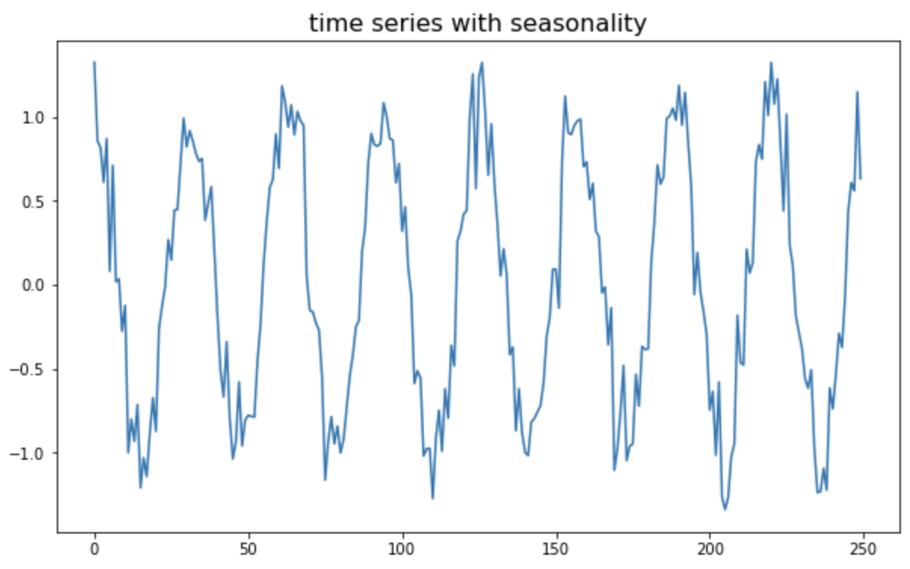
(4-a) ADF 검정 (ADF test)
위의 계절성(seasonality)을 가지는 비정상 시계열에 대해서, ADF 검정(ADF test)을 실시하면, p-value가 3.14e-16 로서 유의수준 5% 하에서 귀무가설(H0: 단위근을 가진다. 즉, 정상 시계열이 아니다)를 기각하고, 대립가설(H1: 단위근을 가지지 않는다. 즉, 정상 시계열이다)를 채택합니다. (땡~! 틀림 -_-;;;)
## checking the stationarity of a series using the ADF(Augmented Dickey-Fuller) Test
# -- Null Hypothesis: The series has a unit root.(not stationary.)
# -- Alternate Hypothesis: The series has no unit root.(stationary.)

adf_test(ts_seasonal) # p-value 3.142783e-16 => stationary (Wrong result. -_-;;;)

# Results of Dickey-Fuller Test:
# Test Statistic                -9.516720e+00
# p-value                        3.142783e-16
# #Lags Used                     1.600000e+01
# Number of Observations Used    2.330000e+02
# Critical Value (1%)           -3.458731e+00
# Critical Value (5%)           -2.874026e+00
# Critical Value (10%)          -2.573424e+00
# dtype: float64
(4-b) KPSS 검정 (KPSS test)
위의 계절성(seasonality)을 가지는 비정상 시계열에 대해서, KPSS 검정(KPSS test)을 실시하면, p-value가 0.1 로서 유의수준 10% 하에서 귀무가설(H0: 정상 시계열이다)를 기각하고, 대립가설(H1: 정상 시계열이 아니다)를 채택합니다. (딩동댕! 맞음 ^_^) (ADF test 는 틀렸고, KPSS test 는 맞았어요. 유의수준 5% 하에서는 둘 다 틀림.)
## KPSS test for checking the stationarity of a time series.
## The null and alternate hypothesis for the KPSS test are opposite that of the ADF test.
# -- Null Hypothesis: The process is trend stationary.
# -- Alternate Hypothesis: The series has a unit root (series is not stationary).

kpss_test(ts_seasonal) # p-value 0.1 => non-stationary (at 10% significance level)

# Results of KPSS Test:
# Test Statistic           0.016014
# p-value                  0.100000
# Lags Used                9.000000
# Critical Value (10%)     0.347000
# Critical Value (5%)      0.463000
# Critical Value (2.5%)    0.574000
# Critical Value (1%)      0.739000
# dtype: float64
이상의 정상성 여부에 대한 통계적 가설 검정 결과를 보면,
(1) 정상 시계열에 대해 ADF test, KPSS test 모두 정상 시계열로 가설 검정 (모두 맞음 ^_^)
(2) 추세가 있는 시계열에 대해 ADF test, KPSS test 가 모두 정상 시계열이 아니라고 정확하게 가설 검정 (모두 맞음 ^_^)
(3) 분산이 변하는 시계열에 대해 ADF test 는 정상 시계열로 가설 검정 (틀렸음! -_-;;;), KPSS test 는 정상 시계열이 아니라고 가설 검정 (맞음 ^_^)
(4) 계절성이 있는 시계열에 대해 ADF test 는 정상 시계열로 가설 검정 (틀렸음! -_-;;;), KPSS test 는 정상 시계열이 아니라고 가설 검정 (맞음 ^_^)
ADF test 는 추세가 있는 비정상 시계열에 대해서는 정상 시계열이 아님을 잘 검정하지만, 분산이 변하거나 계절성이 있는 시계열에 대해서는 정상성 여부를 제대로 검정해내지 못하고 있습니다.
반면에 KPSS test 는 위의 4가지의 모든 경우에 정상성 여부를 잘 검정해내고 있습니다.
통계적 가설 검정 외에 시계열 도표 (time series plot)을 꼭 그려보고 눈으로도 반드시 확인해보는 습관을 들이시기 바랍니다.
[ Reference ]
- ADF test: https://en.wikipedia.org/wiki/Augmented_Dickey%E2%80%93Fuller_test
- KPSS test: https://en.wikipedia.org/wiki/KPSS_test
- ADF test and KPSS test in Python: https://www.statsmodels.org/dev/examples/notebooks/generated/stationarity_detrending_adf_kpss.html
- 단위근 (unit root) : https://www.scienceall.com/%EB%8B%A8%EC%9C%84%EA%B7%BCunit-root-%E5%96%AE%E4%BD%8D%E6%A0%B9/
다음번 포스팅에서는 정상성 가정을 만족하지 않는 시계열 데이터에 대해 데이터 변환을 통해 정상화 시키는 방법을 소개하겠습니다.
이번 포스팅이 많은 도움이 되었기를 바랍니다.
행복한 데이터 과학자 되세요! :-)