R, Python 분석과 프로그래밍의 친구 (by R Friend)

이전 포스팅에서는 

 (i) 정상확률과정(stationary process)의 정의 (https://rfriend.tistory.com/691)

 (ii) 통계적 가설 검증을 통한 시계열 정상성(stationarity test) 여부 확인 (https://rfriend.tistory.com/694)

하는 방법을 소개하였습니다. 

ARIMA 모형과 같은 통계적 시계열 예측 모델의 경우 시계열데이터의 정상성 가정을 충족시켜야 합니다. 따라서 만약 시계열 데이터가 비정상 확률 과정 (non-stationary process) 이라면, 먼저 시계열 데이터 변환을 통해서 정상성(stationarity)을 충족시켜주어야 ARIMA 모형을 적합할 수 있습니다. 

이번 포스팅에서는 Python을 사용하여 

(1) 분산이 고정적이지 않은 경우 분산 안정화 변환 (variance stabilizing transformation, VST)

(2) 추세가 있는 경우 차분을 통한 추세 제거 (de-trend by differencing)

(3) 계절성이 있는 경우 계절 차분을 통한 계절성 제거 (de-seasonality by seaanl differencing)

하는 방법을 소개하겠습니다. 

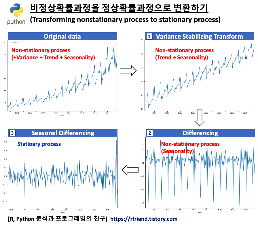
[ 비정상확률과정을 정상확률과정으로 변환하기 (Transforming non-stationary to stationary process) ]

먼저 예제로 사용할 약 판매량 (drug sales) 시계열 데이터를 가져와서 pandas DataFrame으로 만들고, 시계열 그래프를 그려보겠습니다. 

import numpy as np
import pandas as pd
import matplotlib.pyplot as plt 

## getting drug sales dataset 
file_path = 'https://raw.githubusercontent.com/selva86/datasets/master/a10.csv' 
df = pd.read_csv(file_path, 
                 parse_dates=['date'], 
                 index_col='date') 

df.head(12)

#               value
# date	
# 	            3.526591
# 1991-08-01	3.180891
# 1991-09-01	3.252221
# 1991-10-01	3.611003
# 1991-11-01	3.565869
# 1991-12-01	4.306371
# 1992-01-01	5.088335
# 1992-02-01	2.814520
# 1992-03-01	2.985811
# 1992-04-01	3.204780
# 1992-05-01	3.127578
# 1992-06-01	3.270523

## time series plot 
df.plot(figsize=[12, 8]) 
plt.title('Non-Stationary Process: Increasing Variance + Trend + Seasonality', 
          fontsize=16) 
plt.show()

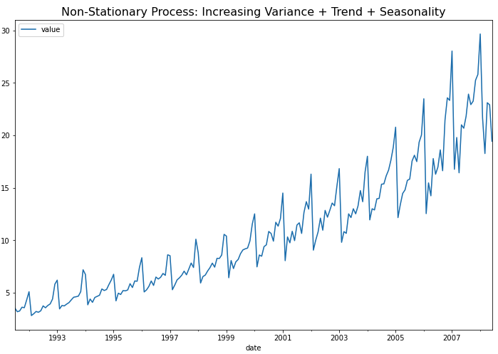
위의 시계열 그래프에서 볼 수 있는 것처럼, (a) 분산이 시간의 흐름에 따라 증가 하고 (분산이 고정이 아님), (b) 추세(trend)가 있으며, (c) 1년 주기의 계절성(seasonality)이 있으므로, 비정상확률과정(non-stationary process)입니다. 

KPSS 검정을 통해서 확인해봐도 p-value가 0.01 이므로 유의수준 5% 하에서 귀무가설 (H0: 정상 시계열이다)을 기각하고, 대립가설(H1: 정상 시계열이 아니다)을 채택합니다. 

## UDF for KPSS test 
from statsmodels.tsa.stattools import kpss 
import pandas as pd 

def kpss_test(timeseries): 
    print("Results of KPSS Test:") 
    kpsstest = kpss(timeseries, regression="c", nlags="auto") 
    kpss_output = pd.Series(
        kpsstest[0:3], index=["Test Statistic", "p-value", "Lags Used"] ) 
    
    for key, value in kpsstest[3].items(): 
        kpss_output["Critical Value (%s)" % key] = value 
    print(kpss_output)
    
    
## 귀무가설 (H0): 정상 시계열이다
## 대립가설 (H1): 정상 시계열이 아니다 <-- p-value 0.01

kpss_test(df)

# Results of KPSS Test:
# Test Statistic           2.013126
# p-value                  0.010000
# Lags Used                9.000000
# Critical Value (10%)     0.347000
# Critical Value (5%)      0.463000
# Critical Value (2.5%)    0.574000
# Critical Value (1%)      0.739000
# dtype: float64

(1) 분산이 고정적이지 않은 경우 분산 안정화 변환 (variance stabilizing transformation, VST)

분산이 고정적이지 않은 경우 멱 변환(Power Transformation)을 통해서 분산을 안정화(variance stabilization) 시켜줍니다. 분산이 고정적이지 않고 추세가 있는 경우 분산 안정화를 추세 제거보다 먼저 해줍니다. 왜냐하면 추세를 제거하기 위해 차분(differencing)을 해줄 때 음수(-)가 생길 수 있기 때문입니다. 

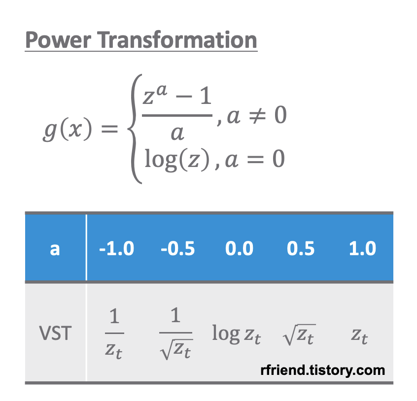
원래의 시계열 데이터의 분산 형태에 따라서 적합한 멱 변환(power transformation)을 선택해서 정상확률과정으로 변환해줄 수 있습니다. 아래의 예제 시도표를 참고하세요. 

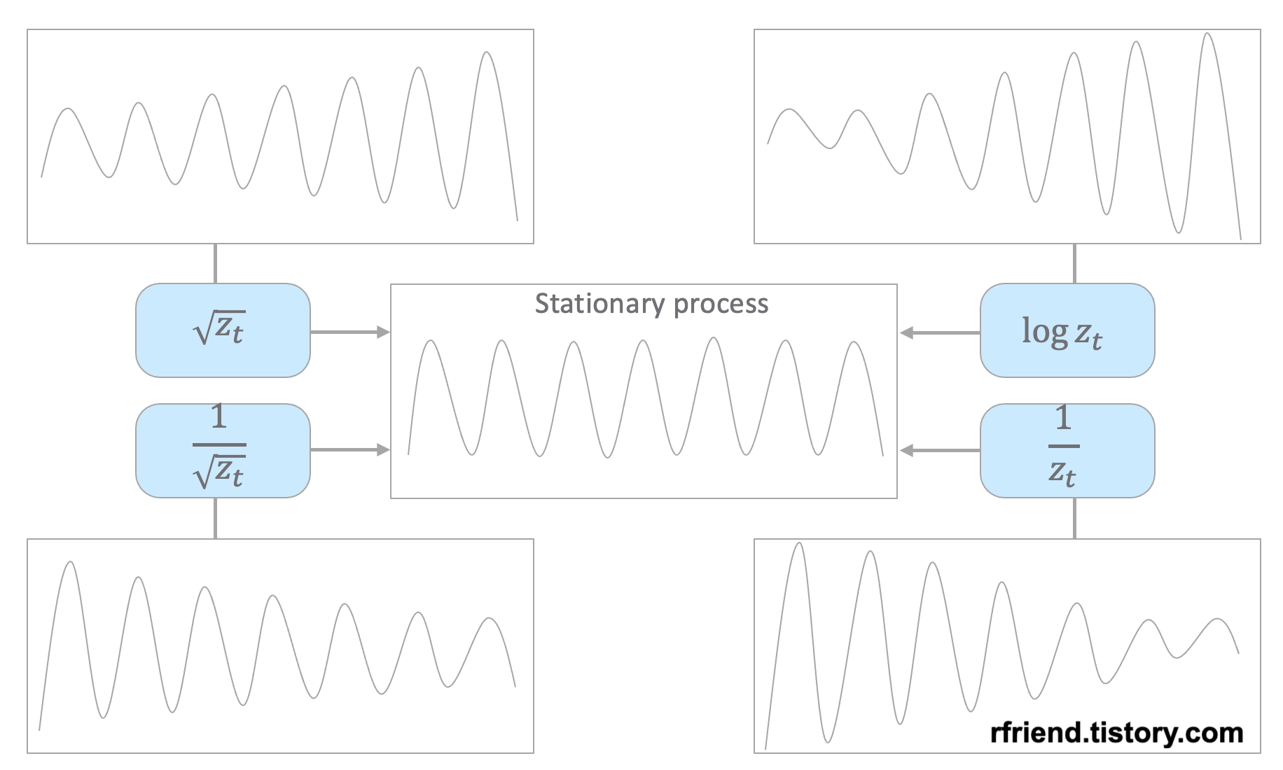
이번 포스팅에서 사용하는 예제는 시간이 흐릴수록 분산이 점점 커지는 형태를 띠고 있으므로 로그 변환(log transformation) 이나 제곱근 변환 (root transformation) 을 해주면 정상 시계열로 변환이 되겠네요. 아래 코드에서는 자연로그를 취해서 로그 변환을 해주었습니다. 

## Variance Stabilizing Transformation (VST) by Taking Logarithm
df_vst = np.log(df.value)

df_vst.head()

# date
# 1991-07-01    1.260332
# 1991-08-01    1.157161
# 1991-09-01    1.179338
# 1991-10-01    1.283986
# 1991-11-01    1.271408
# Name: value, dtype: float64


## plotting
df_vst.plot(figsize=(12, 8))
plt.title("Variance Stabilizing Transformation by taking Logarithm", 
          fontsize=16)
plt.show()

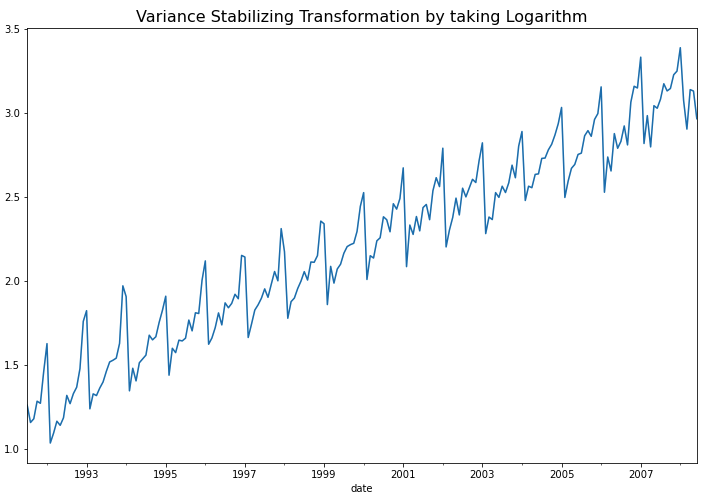
위의 시도표를 보면 시간이 경과해도 분산이 안정화되었음을 알 수 있습니다.  KPSS 검정을 한번 더 해주면 아직 추세(trend)와 계절성(seasonality)가 남아있으므로 여전히 비정상확률과정을 따른다고 나옵니다. 

## 귀무가설 (H0): 정상 시계열이다  
## 대립가설 (H1): 정상 시계열이 아니다  <-- p-value 0.01 

kpss_test(df_vst)

# Results of KPSS Test:
# Test Statistic           2.118189
# p-value                  0.010000
# Lags Used                9.000000
# Critical Value (10%)     0.347000
# Critical Value (5%)      0.463000
# Critical Value (2.5%)    0.574000
# Critical Value (1%)      0.739000
# dtype: float64

(2) 추세가 있는 경우 차분을 통한 추세 제거 (de-trend by differencing)

차분(differencing)은 현재의 시계열 값에서 시차 t 만큼의 이전 값을 빼주는 것입니다. 

1차 차분 = Delta1_Z(t) = Z(t) - Z(t-1) 

2차 차분 = Delta2_Z(t) = Z(t) - Z(t-1) - (Z(t-1) - Z(t-2)) =  Z(t) - 2Z(t-1) + Z(t-2)

Python의 diff() 메소드를 사용해서 차분을 해줄 수 있습니다. 이때 차분의 차수 만큼 결측값이 생기는 데요, dropna() 메소드를 사용해서 결측값은 제거해주었습니다. 

## De-trend by Differencing
df_vst_diff1 = df_vst.diff(1).dropna()

df_vst_diff1.plot(figsize=(12, 8))
plt.title("De-trend by 1st order Differencing", fontsize=16)
plt.show()

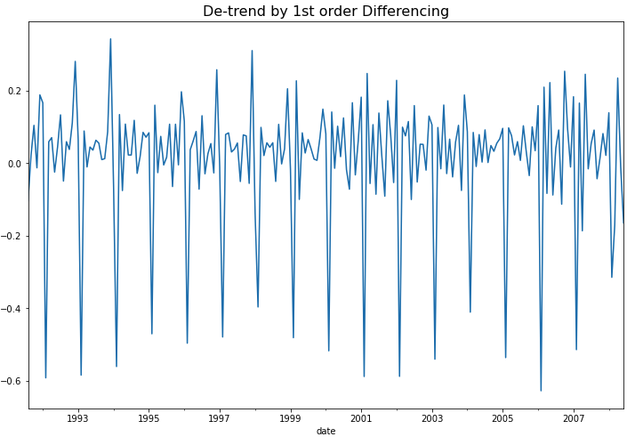
위의 시도표를 보면 1차 차분(1st order differencing)을 통해서 이제 추세(trend)도 제거되었음을 알 수 있습니다. 하지만 아직 계절성(seasonality)이 남아있어서 정상성 조건은 만족하지 않겠네요. 그런데 아래에 KPSS 검정을 해보니 p-value가 0.10 으로서 유의수준 5% 하에서 정상성을 만족한다고 나왔네요. ^^;

## 귀무가설 (H0): 정상 시계열이다  <-- p-value 0.10
## 대립가설 (H1): 정상 시계열이 아니다 

kpss_test(df_vst_diff1)

# Results of KPSS Test:
# Test Statistic            0.121364
# p-value                   0.100000
# Lags Used                37.000000
# Critical Value (10%)      0.347000
# Critical Value (5%)       0.463000
# Critical Value (2.5%)     0.574000
# Critical Value (1%)       0.739000
# dtype: float64

(3) 계절성이 있는 경우 계절 차분을 통한 계절성 제거 (de-seasonality by seaanl differencing)

아직 남아있는 계절성(seasonality)을 계절 차분(seasonal differencing)을 사용해서 제거해보겠습니다. 1년 12개월 주기의 계절성을 띠고 있으므로 diff(12) 함수로 계절 차분을 실시하고, 12개의 결측값이 생기는데요 dropna() 로 결측값은 제거해주었습니다. 

## Stationary Process: De-seasonality by Seasonal Differencing
df_vst_diff1_diff12 = df_vst_diff1.diff(12).dropna()

## plotting
df_vst_diff1_diff12.plot(figsize=(12, 8))
plt.title("De-seasonality by Seasonal Differencing", 
          fontsize=16)
plt.show()

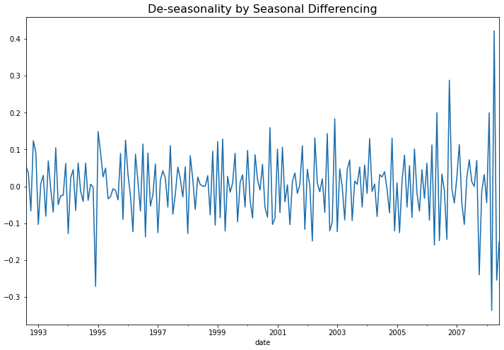
위의 시도표를 보면 이제 계절성도 제거가 되어서 정상 시계열처럼 보이네요. 아래에 KPSS 검정을 해보니 p-value 가 0.10 으로서, 유의수준 5% 하에서 귀무가설(H0: 정상 시계열이다)을 채택할 수 있겠네요.

## 귀무가설 (H0): 정상 시계열이다  <-- p-value 0.10
## 대립가설 (H1): 정상 시계열이 아니다 

kpss_test(df_vst_diff1_diff12)

# Results of KPSS Test:
# Test Statistic           0.08535
# p-value                  0.10000
# Lags Used                8.00000
# Critical Value (10%)     0.34700
# Critical Value (5%)      0.46300
# Critical Value (2.5%)    0.57400
# Critical Value (1%)      0.73900
# dtype: float64

이제 비정상 시계열(non-stationary process)이었던 원래 데이터를 (1) log transformation을 통한 분산 안정화, (2) 차분(differencing)을 통한 추세 제거, (3) 계절 차분(seasonal differencing)을 통한 계절성 제거를 모두 마쳐서 정상 시계열(stationary process) 로 변환을 마쳤으므로, ARIMA 통계 모형을 적합할 수 있게 되었습니다. 

이번 포스팅이 많은 도움이 되었기를 바랍니다. 

행복한 데이터 과학자 되세요!  :-)

지난번 포스팅에서는 NumPy 에서 제공하는

 - (1) 단일 배열 대상의 범용 함수

       (Unary Universal Functions)

 - (2) 2개 배열 대상의 범용 함수

       (Binary Universal Functions)

에 대해서 간략히 소개를 하였습니다.

그리고 단일 배열 대상의 범용 함수 중에서 (1-1) '올림 혹은 내림 (Rounding)' 함수들(np.around, np.round_, np.rint, np.fix, np.ceil, np.floor, np.trunc)에 대해서 알아보았습니다.

이번 포스팅에서는 단일 배열 대상의 범용 함수(Unary ufuncs) 중에서 (1-2) 배열 원소 간 곱(products), 합(sums), 차분(differences) 범용 함수들에 대해서 알아보겠습니다.  (함수가 많아서 한꺼번에 포스팅하기에 버거우므로 여러번 나누어서 포스팅합니다)

[ Unary ufuncs : 배열 원소 간 곱 (products), 합 (sums), 차분 (differences) ]

1차원 배열 b와 2차원 배열 c를 가지고 예를 들어 설명하겠습니다.

2차원 배열의 경우 axis=0 이면 같은 열(column)의 위*아래 방향으로 배열 원소 간 곱하며, axis=1 이면 같은 행(row)의 왼쪽*오른쪽 원소 간 곱을 합니다.

keepdims=True 옵션을 설정하면 1 차원 배열로 배열 원소 간 합을 반환합니다.

2차원 배열의 경우 axis=0 을 설정하면 같은 열(column)의 위+아래 원소 값을 더하며, axis=1 을 설정하면 같은 행(row)의 왼쪽+오른쪽 원소 값을 더하여 1차원 배열을 반환합니다.

np.nanprod() 함수는 NaN (Not a Numbers) 을 '1'(one)로 간주하고 배열 원소 간 곱을 합니다.

np.nansum() 함수는 NaN (Not a Numbers)을 '0'(zero)으로 간주하고 배열 원소 간 더하기를 합니다.

axis=0 이면 같은 행(column)의 위에서 아래 방향으로 배열 원소들을 누적(cumulative)으로 곱해 나가며, axis=1 이면 같은 열(row)에 있는 배열 원소 간에 왼쪽에서 오른쪽 방향으로 누적으로 곱해 나갑니다.

axis=0 이면 같은 행(column)의 위에서 아래 방향으로 배열 원소들을 누적(cumulative)으로 합해 나가며, axis=1 이면 같은 열(row)에 있는 배열 원소 간에 왼쪽에서 오른쪽 방향으로 누적으로 합해 나갑니다.

2차원 배열의 경우 axis=0 이면 같은 열(column)의 아래에서 위 방향으로 차분(difference)을 하며,

axis=1 이면 같은 행(row)의 오른쪽에서 왼쪽 방향으로 차분을 합니다.

2차원 배열에 대한 차분인 np.diff(h, axis=1) 의 경우 Out[38] 처럼 2차원 배열을 반환합니다. 반면에 ediff1d(h) 함수를 사용하면 Out[41] 처럼 차분 결과를 1차원 배열로 반환합니다.

np.ediff1d() 함수의 시작부분과 끝 부분의 값을 to_begin, to_end 로 설정해줄 수도 있습니다.

gradient는 1차 편미분한 값들로 구성된 배열입니다. 아래 예제에 np.gradient() 함수가 어떻게 계산되는지를 수식을 적어놓았으니 참고하시기 바랍니다.  말로 설명하기가 쉽지가 않네요. ^^; 

아래는 2차원 배열에 대한 gradient 구하는 예제입니다. np.gradient(h, axis=0)과 np.gradient(h, axis=1)을 짬뽕해 놓은 것이 np.gradient(h) 라고 보면 되겠습니다.  gradient 방법은 위의 1차원에서 소개한 방법과 같습니다.

다음번 포스팅에서는 지수함수, 로그함수, 삼각함수에 대해서 다루어보겠습니다.

많은 도움 되었기를 바랍니다.