지난번 포스팅에서는 TensorFlow 1.x 버전이 지연(게으른) 실행 (Lazy Execution) 인데 반해 TensorFlow 2.x 버전은 즉시 실행 (Eager Execution) 으로 바뀌었다는 점에 대해서 TenforFlow의 대표적인 자료구조인 상수, 변수, Placeholder 별로 간단한 예를 들어서 비교 설명해 보았습니다. 


이번 포스팅에서는 TensorFlow 2.x 버전에서 크게 바뀐 것 중에서 "고수준 API (High-Level API) 로서 Keras API를 채택"하였다는 것에 대해서 소개하겠습니다. 


TensorFlow 2.x 는 텐서 연산은 C++로 고속으로 수행하며, 저수준 API에는 Python wrapper 의 TensorFlow가 있고, 고수준 API로는 Keras 를 사용하는 아키텍처입니다. Keras도 당연히 CPU 뿐만 아니라 GPU 를 사용한 병렬처리 학습이 가능하며, 다양한 애플리케이션/디바이스에 배포도 가능합니다. 


Keras는 Google 에서 딥러닝 연구를 하고 있는 Francois Chollet 이 만든 Deep Learning Library 인데요, TensorFlow 2.x 버전에 고수준 API 로 포함이 되었습니다. (고마워요 Google!!!)


TensorFlow 1.x 버전을 사용할 때는 TensorFlow 설치와 별도로 Native Keras를 따로 설치하고 또 Keras를 별도로 import 해서 사용해야 했습니다. 


하지만 TensorFlow 2.x 버전 부터는 TensorFlow 만 설치하면 되며, Keras는 별도로 설치하지 않아도 됩니다. 또한 Keras API를 사용할 때도 TensorFlow를 Importing 한 후에 tf.keras.models 와 같이 tf.keras 로 시작해서 뒤에 Keras의 메소드를 써주면 됩니다. (아래의 MNIST 분류 예시에서 자세히 소개)


TensorFlow 1.x 

TensorFlow 2.x 

 설치 (Install)

 $ pip install tensorflow==1.15

 $ pip install keras

 $ pip install tensorflow==2.3.0 

 (Keras는 별도 설치 필요 없음)

 Importing

 import tensorflow as tf

from keras import layers

 import tensorflow as tf

 from tf.keras import layers


위의 Kreas 로고 이미지는 https://keras.io 정식 홈페이지의 메인 화면에 있는 것인데요, "Simple. Flexible. Powerful." 가 Keras의 모토이며, Keras를 아래처럼 소개하고 있습니다. 


"Keras는 TensorFlow 기계학습 플랫폼 위에서 실행되는 Python 기반의 딥러닝 API 입니다. Keras는 빠른 실험을 가능하게 해주는데 초점을 두고 개발되었습니다. 아이디어에서부터 결과를 얻기까지 가능한 빠르게 할 수 있다는 것은 훌륭한 연구를 하는데 있어 매우 중요합니다" 

* Keras reference: https://keras.io/about/


백문이 불여일견이라고, Keras를 사용하여 MNIST 손글씨 0~9 숫자를 분류하는 매우 간단한 DNN (Deep Neural Network) 모델을 만들어보겠습니다.


DNN Classifier 모델 개발 및 적용 예시는 (1) 데이터 준비, (2) 모델 구축, (3) 모델 컴파일, (4) 모델 학습, (5) 모델 평가, (6) 예측의 절차에 따라서 진행하겠습니다. 


[ MNIST 데이터 손글씨 숫자 분류 DNN 모델 ]


  (1) 데이터 준비 (Preparing the data)


먼저 TensorFlow 를 importing 하고 버전(TensorFlow 2.3.0)을 확인해보겠습니다. 


import tensorflow as tf

import numpy as np


print(tf.__version__)

2.3.0


Keras 에는 MNIST 데이터셋이 내장되어 있어서 tf.keras.datasets.mnist.load_data() 메소드로 로딩을 할 수 있습니다. Training set에 6만개, Test set에 1만개의 손글씨 숫자 데이터와 정답지 라벨 데이터가 있습니다. 


(x_train, y_train), (x_test, y_test) = tf.keras.datasets.mnist.load_data()


print('shape of x_train:', x_train.shape)

print('shape of y_train:', y_train.shape)

print('shape of x_test:', x_test.shape)

print('shape of y_test:', y_test.shape)

shape of x_train: (60000, 28, 28)
shape of y_train: (60000,)
shape of x_test: (10000, 28, 28)
shape of y_test: (10000,)


 MNIST 데이터셋이 어떻게 생겼는지 확인해보기 위해서 Training set의 0번째 이미지 데이터 배열(28 by 28 array)과 정답지 라벨 ('5'), 그리고 matplotlib 으로 시각화를 해보겠습니다. 


x_train[0]

[Out] array([[ 0, 0, 0, 0, 0, 0, 0, 0, 0, 0, 0, 0, 0, 0, 0, 0, 0, 0, 0, 0, 0, 0, 0, 0, 0, 0, 0, 0], [ 0, 0, 0, 0, 0, 0, 0, 0, 0, 0, 0, 0, 0, 0, 0, 0, 0, 0, 0, 0, 0, 0, 0, 0, 0, 0, 0, 0], [ 0, 0, 0, 0, 0, 0, 0, 0, 0, 0, 0, 0, 0, 0, 0, 0, 0, 0, 0, 0, 0, 0, 0, 0, 0, 0, 0, 0], [ 0, 0, 0, 0, 0, 0, 0, 0, 0, 0, 0, 0, 0, 0, 0, 0, 0, 0, 0, 0, 0, 0, 0, 0, 0, 0, 0, 0], [ 0, 0, 0, 0, 0, 0, 0, 0, 0, 0, 0, 0, 0, 0, 0, 0, 0, 0, 0, 0, 0, 0, 0, 0, 0, 0, 0, 0], [ 0, 0, 0, 0, 0, 0, 0, 0, 0, 0, 0, 0, 3, 18, 18, 18, 126, 136, 175, 26, 166, 255, 247, 127, 0, 0, 0, 0], [ 0, 0, 0, 0, 0, 0, 0, 0, 30, 36, 94, 154, 170, 253, 253, 253, 253, 253, 225, 172, 253, 242, 195, 64, 0, 0, 0, 0], [ 0, 0, 0, 0, 0, 0, 0, 49, 238, 253, 253, 253, 253, 253, 253, 253, 253, 251, 93, 82, 82, 56, 39, 0, 0, 0, 0, 0], [ 0, 0, 0, 0, 0, 0, 0, 18, 219, 253, 253, 253, 253, 253, 198, 182, 247, 241, 0, 0, 0, 0, 0, 0, 0, 0, 0, 0], [ 0, 0, 0, 0, 0, 0, 0, 0, 80, 156, 107, 253, 253, 205, 11, 0, 43, 154, 0, 0, 0, 0, 0, 0, 0, 0, 0, 0], [ 0, 0, 0, 0, 0, 0, 0, 0, 0, 14, 1, 154, 253, 90, 0, 0, 0, 0, 0, 0, 0, 0, 0, 0, 0, 0, 0, 0], [ 0, 0, 0, 0, 0, 0, 0, 0, 0, 0, 0, 139, 253, 190, 2, 0, 0, 0, 0, 0, 0, 0, 0, 0, 0, 0, 0, 0], [ 0, 0, 0, 0, 0, 0, 0, 0, 0, 0, 0, 11, 190, 253, 70, 0, 0, 0, 0, 0, 0, 0, 0, 0, 0, 0, 0, 0], [ 0, 0, 0, 0, 0, 0, 0, 0, 0, 0, 0, 0, 35, 241, 225, 160, 108, 1, 0, 0, 0, 0, 0, 0, 0, 0, 0, 0], [ 0, 0, 0, 0, 0, 0, 0, 0, 0, 0, 0, 0, 0, 81, 240, 253, 253, 119, 25, 0, 0, 0, 0, 0, 0, 0, 0, 0], [ 0, 0, 0, 0, 0, 0, 0, 0, 0, 0, 0, 0, 0, 0, 45, 186, 253, 253, 150, 27, 0, 0, 0, 0, 0, 0, 0, 0], [ 0, 0, 0, 0, 0, 0, 0, 0, 0, 0, 0, 0, 0, 0, 0, 16, 93, 252, 253, 187, 0, 0, 0, 0, 0, 0, 0, 0], [ 0, 0, 0, 0, 0, 0, 0, 0, 0, 0, 0, 0, 0, 0, 0, 0, 0, 249, 253, 249, 64, 0, 0, 0, 0, 0, 0, 0], [ 0, 0, 0, 0, 0, 0, 0, 0, 0, 0, 0, 0, 0, 0, 46, 130, 183, 253, 253, 207, 2, 0, 0, 0, 0, 0, 0, 0], [ 0, 0, 0, 0, 0, 0, 0, 0, 0, 0, 0, 0, 39, 148, 229, 253, 253, 253, 250, 182, 0, 0, 0, 0, 0, 0, 0, 0], [ 0, 0, 0, 0, 0, 0, 0, 0, 0, 0, 24, 114, 221, 253, 253, 253, 253, 201, 78, 0, 0, 0, 0, 0, 0, 0, 0, 0], [ 0, 0, 0, 0, 0, 0, 0, 0, 23, 66, 213, 253, 253, 253, 253, 198, 81, 2, 0, 0, 0, 0, 0, 0, 0, 0, 0, 0], [ 0, 0, 0, 0, 0, 0, 18, 171, 219, 253, 253, 253, 253, 195, 80, 9, 0, 0, 0, 0, 0, 0, 0, 0, 0, 0, 0, 0], [ 0, 0, 0, 0, 55, 172, 226, 253, 253, 253, 253, 244, 133, 11, 0, 0, 0, 0, 0, 0, 0, 0, 0, 0, 0, 0, 0, 0], [ 0, 0, 0, 0, 136, 253, 253, 253, 212, 135, 132, 16, 0, 0, 0, 0, 0, 0, 0, 0, 0, 0, 0, 0, 0, 0, 0, 0], [ 0, 0, 0, 0, 0, 0, 0, 0, 0, 0, 0, 0, 0, 0, 0, 0, 0, 0, 0, 0, 0, 0, 0, 0, 0, 0, 0, 0], [ 0, 0, 0, 0, 0, 0, 0, 0, 0, 0, 0, 0, 0, 0, 0, 0, 0, 0, 0, 0, 0, 0, 0, 0, 0, 0, 0, 0], [ 0, 0, 0, 0, 0, 0, 0, 0, 0, 0, 0, 0, 0, 0, 0, 0, 0, 0, 0, 0, 0, 0, 0, 0, 0, 0, 0, 0]], dtype=uint8)


y_train[0]

[Out] 5


import matplotlib.pyplot as plt

plt.rcParams['figure.figsize'] = (5, 5)

plt.imshow(x_train[0])

plt.show()


Deep Neural Network 모델의 input으로 넣기 위해 (28 by 28) 2차원 배열 (2D array) 이미지를 (28 * 28 = 784) 의 옆으로 길게 펼친 데이터 형태로 변형(Reshape) 하겠습니다(Flatten() 메소드를 사용해도 됨). 그리고 0~255 사이의 값을 0~1 사이의 실수 값으로 변환하겠습니다.  


# reshape and normalization

x_train = x_train.reshape((60000, 28 * 28)) / 255.0

x_test = x_test.reshape((10000, 28 * 28)) / 255.0


  (2) 모델 구축 (Building the model)


이제 본격적으로 Keras를 사용해보겠습니다. Keras의 핵심 데이터 구조로 모델(Models)층(Layers)있습니다. 모델을 구축할 때는 (a) 순차적으로 층을 쌓아가는 Sequential model 과, (b) 복잡한 구조의 모델을 만들 때 사용하는 Keras functional API 의 두 가지 방법이 있습니다. 


이미지 데이터 분류는 CNN (Convolutional Neural Network) 을 사용하면 효과적인데요, 이번 포스팅에서는 간단하게 Sequential model 을 사용하여 위의 (1)에서 전처리한 Input 이미지 데이터를 받아서, 1개의 완전히 연결된 은닉층 (Fully Connected Hidden Layer) 을 쌓고, 10개의 classes 별 확률을 반환하는 FC(Fully Connected) Output Layer 를 쌓아서 만든 DNN(Deep Neural Network) 모델을 만들어보겠습니다.  (Functional API 는 PyTorch 와 유사한데요, 나중에 별도의 포스팅에서 소개하도록 하겠습니다.)


add() 메소드를 사용하면 마치 레고 블록을 쌓듯이 차곡차곡 순서대로 원하는 층을 쌓아서 딥러닝 모델을 설계할 수 있습니다. (Dense, CNN, RNN, Embedding 등 모두 가능). Dense() 층의 units 매개변수에는 층별 노드 개수를 지정해주며, 활성화 함수는 activation 매개변수에서 지정해줍니다. 은닉층에서는 'Relu' 활성화함수를, Output 층에는 10개 classes에 대한 확률을 반환하므로 'softmax' 활성화함수를 사용하였습니다. 


# Sequential model

model = tf.keras.models.Sequential()


# Stacking layers

model.add(tf.keras.layers.Dense(units=128, activation='relu', input_shape=(28*28,)))

model.add(tf.keras.layers.Dense(units=10, activation='softmax'))


이렇게 층을 쌓아서 만든 DNN (Deep Neural Network) 모델이 어떻게 생겼는지 summary() 함수로 출력해보고, tf.keras.utils.plot_model() 메소드로 시각화해서 확인해보겠습니다. 


model.summary()

Model: "sequential"
_________________________________________________________________
Layer (type)                 Output Shape              Param #   
=================================================================
dense (Dense)                (None, 128)               100480    
_________________________________________________________________
dense_1 (Dense)              (None, 10)                1290      
=================================================================
Total params: 101,770
Trainable params: 101,770
Non-trainable params: 0
_____________________________________


# keras model visualization

tf.keras.utils.plot_model(model, 

                          to_file='model_plot.png', 

                          show_shapes=True)


* 참고로 Keras의 tf.keras.utils.plot_model() 메소드를 사용하려면 사전에 pydot, pygraphviz 라이브러리 설치, Graphviz 설치가 필요합니다. 


  (3) 모델 컴파일 (Compiling the model)


위의 (2)번에서 딥러닝 모델을 구축하였다면, 이제 기계가 이 모델을 이해할 수 있고 학습 절차를 설정할 수 있도록 컴파일(Compile) 해줍니다. 


compile() 메소드에는 딥러닝 학습 시 사용하는 (a) 오차 역전파 경사하강법 시 최적화 알고리즘(optimizer), (b) 손실함수(loss function), 그리고 (c) 성과평가 지표(metrics) 를 설정해줍니다. 


model.compile(optimizer='sgd', 

              loss='sparse_categorical_crossentropy', 

              metrics=['accuracy']

)


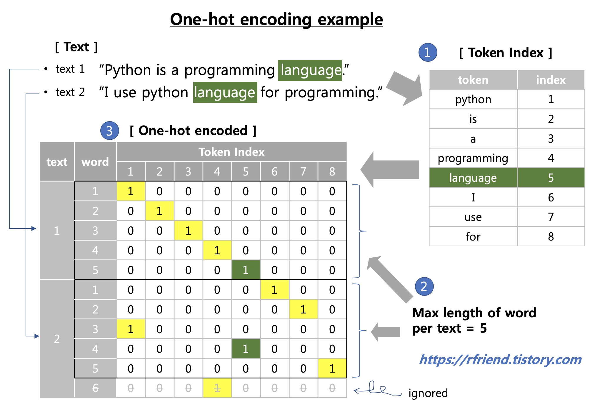
* 참고로, input data의 다수 클래스에 대한 정답 레이블(ground-truth labels)을 바로 사용하여 손실함수를 계산할 때는 loss='sparse_categorical_crossentropy' 을 사용하며, One-hot encoding 형태로 정답 레이블이 되어있다면 loss='categorical_crossentropy' 를 사용합니다. 


Keras 는 위에서 처럼 optimizer='sgd' 처럼 기본 설정값을 사용해서 간단하게 코딩할수도 있으며, 만약 사용자가 좀더 유연하고 강력하게 설정값을 조정하고 싶다면 아래의 예시처럼 하위클래스(subclassing)을 사용해서 세부 옵션을 지정해줄 수도 있습니다. 


model.compile(

    optimizer=keras.optimizers.SGD(learning_rate=0.01, momentum=0.9, nesterov=True)

    loss=keras.losses.sparse_categorical_crossentropy

)


  (4) 모델 학습 (Training the model)


데이터 준비와 모델 구축, 그리고 모델 컴파일이 끝났으므로 이제 6만개의 훈련 데이터셋(Training set) 중에서 80% (4.8만개 데이터) 는 모델 학습(fitting)에, 20%(1.2만개 데이터)는 검증(validation)용으로 사용하여 DNN 모델을 학습해보겠습니다. (참고로, 1만개의 Test set은 모델 학습에서는 사용하지 않으며, 최종 모델에 대해서 제일 마지막에 모델 성능 평가를 위해서만 사용합니다.)


epochs = 5 는 전체 데이터를 5번 반복(iteration)해서 사용해서 학습한다는 의미입니다. 

verbose = 1 은 모델 학습 진행상황 막대를 출력하라는 의미입니다. ('1' 이 default이므로 생략 가능)

(0 = silent, 1 = progress bar, 2 = one line per epoch)

validation_split=0.2 는 검증용 데이터셋을 별도로 만들어놓지 않았을 때 학습용 데이터셋에서 지정한 비율(예: 20%) 만큼을 분할하여 (hyperparameter tuning을 위한) 검증용 데이터셋으로 이용하라는 의미입니다. 

batch_size=32 는 한번에 데이터 32개씩 batch로 가져다가 학습에 사용하라는 의미입니다. 


이번 포스팅은 Keras의 기본 사용법에 대한 개략적인 소개이므로 너무 자세하게는 안들어가겠구요, callbacks는 나중에 별도의 포스팅에서 자세히 설명하겠습니다. 


학습이 진행될수록 (즉, epochs 이 증가할 수록) 검증용 데이터셋에 대한 손실 값(loss value)은 낮아지고 정확도(accuracy)는 올라가고 있네요. 


model.fit(x_train, y_train, 

          epochs=5, 

          verbose=1, 

          validation_split=0.2)


Epoch 1/5
1500/1500 [==============================] - 1s 922us/step - loss: 0.7291 - accuracy: 0.8146 - val_loss: 0.3795 - val_accuracy: 0.8989
Epoch 2/5
1500/1500 [==============================] - 1s 811us/step - loss: 0.3605 - accuracy: 0.9007 - val_loss: 0.3081 - val_accuracy: 0.9145
Epoch 3/5
1500/1500 [==============================] - 1s 785us/step - loss: 0.3061 - accuracy: 0.9140 - val_loss: 0.2763 - val_accuracy: 0.9215
Epoch 4/5
1500/1500 [==============================] - 1s 772us/step - loss: 0.2749 - accuracy: 0.9228 - val_loss: 0.2519 - val_accuracy: 0.9290
Epoch 5/5
1500/1500 [==============================] - 1s 827us/step - loss: 0.2525 - accuracy: 0.9289 - val_loss: 0.2355 - val_accuracy: 0.9339
Out[14]:
<tensorflow.python.keras.callbacks.History at 0x7fc7920a1760>


  (5) 모델 평가 (Evaluating the model)


evaluate() 메소드를 사용하여 모델의 손실 값(Loss value) 과 컴파일 단계에서 추가로 설정해준 성능지표 값 (Metrics values) 을 Test set 에 대하여 평가할 수 있습니다. (다시 한번 강조하자면, Test set은 위의 (4)번 학습 단계에서 절대로 사용되어서는 안됩니다!)


Test set에 대한 cross entropy 손실값은 0.234, 정확도(accuracy)는 93.68% 가 나왔네요. (CNN 모델을 이용하고 hyperparameter tuning을 하면 99%까지 정확도를 올릴 수 있습니다.)


model.evaluate(x_test, y_test)

313/313 [==============================] - 0s 801us/step - loss: 0.2342 - accuracy: 0.9368
Out[15]:
[0.23418554663658142, 0.9368000030517578]


  (6) 예측 (Prediction for new data) 


위에서 학습한 DNN 모델을 사용해서 MNIST 이미지 데이터에 대해서 predict() 메소드를 사용하여 예측을 해보겠습니다. (별도의 새로운 데이터가 없으므로 test set 데이터를 사용함)


예측 결과의 0번째 데이터를 살펴보니 '7' 이라고 모델이 예측을 했군요. 


preds = model.predict(x_test, batch_size=128)


# returns an array of probability per classes

preds[0]

array([8.6389220e-05, 3.9117887e-07, 5.6002376e-04, 2.2136024e-03,
       2.7992455e-06, 1.4370076e-04, 5.6979918e-08, 9.9641860e-01,
       2.2985958e-05, 5.5149395e-04], dtype=float32)


# position of max probability

np.argmax(preds[0])

[Out] 7


실제 정답 레이블(ground-truth labels)과 비교해보니 '7' 이 정답이 맞네요. 


y_test[0]

[Out] 7


plt.imshow(x_test[0].reshape(28, 28))

plt.show()


  (7) 모델 저장, 불러오기 (Saving and Loading the model)


딥러닝 모델의 성과 평가 결과 기준치를 충족하여 현장 적용이 가능한 경우라면 모델의 요소와 학습된 가중치 정보를 파일 형태로 저장하고, 배포, 로딩해서 (재)활용할 수 있습니다. 


-  HDF5 파일로 전체 모델/가중치 저장하기


# Save the entire model to a HDF5 file.

model.save('mnist_dnn_model.h5') 


- 저장된 'mnist_dnn_model.h5' 모델/가중치 파일을 'new_model' 이름으로 불러오기


# Recreate the exact same model, including its weights and the optimizer

new_model = tf.keras.models.load_model('mnist_dnn_model.h5')


new_model.summary()

Model: "sequential"
_________________________________________________________________
Layer (type)                 Output Shape              Param #   
=================================================================
dense (Dense)                (None, 128)               100480    
_________________________________________________________________
dense_1 (Dense)              (None, 10)                1290      
=================================================================
Total params: 101,770
Trainable params: 101,770
Non-trainable params: 0
_________________________________________________________________


TensorFlow 2.x 에서부터 High-level API 로 탑재되어 있는 Keras API 에 대한 간단한 MNIST 분류 DNN 모델 개발과 예측 소개를 마치겠습니다. 


* About Kerashttps://keras.io/about/

* Keras API Reference: https://keras.io/api/

* Save and Load model: https://www.tensorflow.org/tutorials/keras/save_and_load


많은 도움이 되었기를 바랍니다. 

이번 포스팅이 도움이 되었다면 아래의 '공감~'를 꾹 눌러주세요. :-)


728x90
반응형
Posted by Rfriend
,

2019년도 9월 말에 TensorFlow 2.0 버전이 공개되었으며. 이전의 TensorFlow 1.x 대비 (1) API Cleanup, (2) Eager execution, (3) No more globals, (4) Functions, not sessions 와 같은 변화가 있었습니다. (https://www.tensorflow.org/guide/effective_tf2)


이번 포스팅에서는 TensorFlow 1.x 에서의 지연 실행모드(Lazy execution), Global namespace, Session 호출 대비, TensorFlow 2.x 에서  Global namespace 나 Session 호출 없이, 즉시 실행모드(Eager execution)에 대해서 간단한 예제를 들어서 비교 설명해보겠습니다. 

(Keras API 와의 통합은 다음번 포스팅에서 소개하겠습니다.)


아래 비교 예제를 살펴보면 TensorFlow 2.x 에서의 코드가 한결 깔끔해져서 가독성도 좋아지고, 디버깅하기에도 편리해졌음을 알 수 있을 겁니다.  Python 프로그리밍에 이미 익숙한 사용자라면 TensorFlow 2.x 버전이 사용하기에 무척 친숙하게 느껴질 것입니다. 


아래에는 TensorFlow 1.12.0 버전과 TensorFlow 2.3.0 버전을 사용하여 TensorFlow 의 핵심 데이터 구조인 상수(constant), 변수(Variable), Placeholder 로 나누어서 TensorFlow 버전 간 비교해보겠습니다. 


  (1) 상수 (constant) 생성 및 연산 실행


 TensorFlow 1.x: 지연 실행 (lazy execution)

TensorFlow 2.x: 즉시 실행 (eager execution)


import tensorflow as tf


tf.__version__

'1.12.0'


a = tf.constant([0, 1, 2])

b = tf.constant([10, 20, 30])


# lazy execution

c = tf.add(a, b)

print(c)

Tensor("Add:0", shape=(3,), 
dtype=int32)


with tf.Session() as sess:

    print(sess.run(c))


[10 21 32]


import tensorflow as tf


tf.__version__

'2.3.0'


a = tf.constant([0, 1, 2])

b = tf.constant([10, 20, 30])


# eager execution

c = tf.add(a, b) # or c = a + b

print(c)

tf.Tensor([10 21 32], 
shape=(3,), dtype=int32)


TensorFlow 1.x 버전에서는 지연 실행 모드 (lazy execution) 가 기본 설정이므로 위의 더하기(add) 예제에서처럼 tf.constant() 로 두 개의 상수 배열을 만들고, tf.add(a, b)를 하면 바로 실행되는 것이 아니며, 계산 그래프와 Session을 생성하고 명시적으로 tf.Session().run() 을 호출하고 나서야 연산이 실행됩니다. 


반면에 TensorFlow 2.x 버전에서는 즉시 실행 모드 (eager execution) 가 기본 설정이므로 a, b 의 두 상수 배열을 생성한 후 tf.add(a, b) 를 하면 Session().run() 없이 바로 더하기 연산이 실행되어 그 결과를 반환합니다. 


TensorFlow 2.x 에서는 아래의 예처럼 numpy() 메소드를 사용해서 텐서를 numpy array 로 변환하여 텐서의 값에 접근할 수 있습니다. (참고로, 반대로 tf.convert_to_tensor(arr) 메소드를 사용하면 numpy array를 텐서 값으로 변환할 수 있습니다.)


# TensorFlow 2.x

# accessing the value of a Tensor

c_arr = c.numpy()

print(c_arr)

[10 21 32]


  (2) 변수 (Variable) 생성 및 연산 실행


TensorFlow 1.x

: lazy execution, session, global namespaces

TensorFlow 2.x

: eager execution, no session, no globals


import tensorflow as tf


tf.__version__

'1.12.0'


w = tf.Variable([[1.], [2.]])

x = tf.constant([[3., 4.]])


print(w)

<tf.Variable 'Variable:0' shape=(2, 1) dtype=float32_ref>


print(x)
Tensor("Const_2:0", shape=(1, 2), 
dtype=float32)


# lazy execution

w_x_matmul = tf.matmul(w, x)

print(w_x_matmul)

Tensor("MatMul:0", shape=(2, 2), 
dtype=float32)


with tf.Session() as sess:
    # initialization of variable
    sess.run(tf.global_variables_initializer())
    
    # runn tf.Session
    print(sess.run(w_x_matmul))


[[3. 4.]
 [6. 8.]]


import tensorflow as tf


tf.__version__

'2.3.0'


w = tf.Variable([[1.], [2.]])

x = tf.constant([[3., 4.]]) 


print(w)

<tf.Variable 'Variable:0' shape=(2, 1) dtype=float32, numpy=
array([[1.],
       [2.]], dtype=float32)>


print(x)

tf.Tensor([[3. 4.]], shape=(1, 2), 
dtype=float32)


# eager execution

# no need for tf.global_variables_initializer()

w_x_matmul = tf.matmul(w, x)

print(w_x_matmul)

tf.Tensor(
[[3. 4.]
 [6. 8.]], shape=(2, 2), 
dtype=float32)


tf.Variable() 로 생성한 w 변수(Variable)와 tf.constant()로 생성한 상수로 tf.matmul() 메소드로 행렬곱 연산을 수행하여 보았습니다. 


TensorFlow 1.x 버전에서는 지연 연산 (lazy execution) 모드이므로 tf.matmul(w, x) 에서는 아무런 연산이 일어나지 않으며, Session을 열고 session.run()으로 명시적으로 호출할 때에야 비로서 행렬곱 연산이 실행됩니다. 더불어서, 변수를 Session 에서 실행시키기 전에 tf.global_variables_initializer() 를 먼저 호출해서 변수를 초기화(initialization) 해주어야 합니다. 


반면에 TensorFlow 2.x 버전에서는 tf.Variable(), tf.constant() 로 값을 할당해주면 바로 실행이 되어 변수와 상수가 생성이 됩니다. 그리고 tf.matmul() 메소드로 행렬곱 연산을 즉시 수행하여 결과값을 반환받습니다. (이때 tf.global_variables_initializer() 를 호출할 필요는 없습니다.) TenforFlow 1.x 대비 TensorFlow 2.x 가 코드가 한결 깔끔해졌습니다. 


  (3) tf.placeholder(...), feed_dict


Placeholder 는 TensorFlow에서 그래프를 실행할 때 사용자가 데이터를 주입할 수 있는 통로입니다. TensforFlow 1.x 버전에서는 아래처럼 Session을 실행할 때 feed_dict 매개변수를 사용하여 feed_dict = {placeholder: input} 처럼 사전형으로 값을 입력할 수 있습니다. 

반면에 TensorFlow 2.x 버전에서는 Session() 실행없이 바로 함수(function)에 입력값(input)을 넣어서 즉시 실행할 수 있습니다. 역시 코드가 한결 깔끔해졌습니다. 


# TensorFlow 1.x

outputs = session.run(f(placeholder), feed_dict={placeholder: input})


# TensorFlow 2.x

outputs = f(input)


TensorFlow 1.x:

Session, Placeholder & feed_dict 

 TensorFlow 2.x:

function


import tensorflow as tf


tf.__version__

'1.12.0'


# placeholder

a = tf.placeholder(tf.int32)

b = tf.placeholder(tf.int32)


# defining a summation function

def tf_sum(a, b):

    return a + b


# lazy execution

a_b_sum = tf_sum(a, b)


print(a_b_sum)

Tensor("add_1:0", dtype=int32)


with tf.Session() as sess:

    print(sess.run(a_b_sum, 

                  feed_dict = {a: [0, 1, 2], 

                               b: [10, 20, 30]}))


[10 21 32]


import tensorflow as tf


tf.__version__

'2.3.0'


a = tf.constant([0, 1, 2])

b = tf.constant([10, 20, 30])


# define a summation fuction

def tf_sum(a, b):

    return a + b


# eager execution

a_b_sum = tf_sum(a, b)


print(a_b_sum)

tf.Tensor([10 21 32], shape=(3,), 
dtype=int32)


많은 도움이 되었기를 바랍니다. 

이번 포스팅이 도움이 되었다면 아래의 '공감~'를 꾹 눌러주세요. 


728x90
반응형
Posted by Rfriend
,

이번 포스팅에서는 Python의 NLTK (Natural Language Toolkit) 라이브러리WordNet 말뭉치를 사용하여 자연어 처리 (Natural Language Processing) 하는 몇 가지 방법을 맛보기로 소개하겠습니다. 

(저는 Python 3.8 버전에 NLTK 3.5 버전을 사용하였습니다. 자연어 처리, NLTK를 제대로 살펴보려면 책 한권, 한 학기 수업 분량이며, 이번 포스팅은 말 그대로 맛보기 정도의 소개입니다. ^^;)


Python NLTK (Natural Language Toolkit) 라이브러리는 텍스트 분류, 토큰화, 단어 stemming, 품사 태킹, 텍스트 파싱, semantic reasoning 등을 하는데 사용하는 텍스트 자연어 처리 파이썬 모듈입니다.

(* reference: https://www.nltk.org/book/ch02.html )


WordNet은 어휘에 중점을 둔 영어 사전 Database 로서, 전통적인 Thesaurus (유의어 사전)와 유사한 측면이 있지만 보다 풍성한 구조를 가지고 있습니다. 1985년부터 프린스턴 대학교에서 구축하기 시작하였으며, 약 16만개의 단어(155287 words)와 12만개의 유사어 집합(117,659 synonym sets)을 포함하고 있는 방대한 Thesaurus 입니다. 

(* reference: https://www.nltk.org/howto/wordnet.html )


NLTK와 WordNet에 대한 간단한 소개를 마쳤으니 이제 직접 코드를 짜보면서 예를 들어보겠습니다. 먼저, 명령 프롬프트 창에서 pip install로 NLTK 라이브러리를 설치하고 pip show로 버전과 내용을 확인해보겠습니다. (Anaconda 배포판으로 Python 가상 환경을 만들었다면 아마 디폴트로 NLTK 모듈이 설치되어 있을 겁니다.)


-- (명령 프롬프트 창에서) NLTK 모듈 설치

$ pip install nltk


-- NLTK 모듈 확인

$ pip show nltk

Name: nltk

Version: 3.5

Summary: Natural Language Toolkit

Home-page: http://nltk.org/

Author: Steven Bird

Author-email: stevenbird1@gmail.com

License: Apache License, Version 2.0

Location: /Users/ihongdon/anaconda3/envs/py3.8_tf2.3/lib/python3.8/site-packages

Requires: regex, click, tqdm, joblib

Required-by: 


 (1) NLTK로 Word Tokenization 하기


Token 이란 더이상 나눌 수 없는 언어요소를 말하며, Tokenization은 텍스트 문자열을 Token으로 분해하여 쪼개는 것입니다. 


처음 사용하는 경우라면 먼저 nltk.download('punkt') 를 실행하여 Punket Tokenizer Models (13MB) 를 다운로드 해줍니다. 


nltk.word_tokenize() 함수를 사용해서 괄호 안에 텍스트 문자열 객체를 넣어주면 Token으로 쪼개줍니다. 

(영어는 띄어쓰기 기준으로 단어 토큰화가 되었는데요, 한글은 단순히 띄어쓰기 기준만으로 토큰화가 되지 않는 어려움이 있습니다.)


#%% word tokenization


import nltk


# Please use the NLTK Downloader to obtain the resource:

nltk.download('punkt')


sentense = "NLTK is a leading platform for building Python programs to work with human language data."


tokens = nltk.word_tokenize(sentense)

tokens

Out[1]: 

['NLTK',

 'is',

 'a',

 'leading',

 'platform',

 'for',

 'building',

 'Python',

 'programs',

 'to',

 'work',

 'with',

 'human',

 'language',

 'data',

 '.']


* 참고로, keras 라이브러리로의 text_to_word_seqence() 메소드로 단어 토큰화를 할 수 있습니다. 

(from tensorflow.keras.preprocessing.text import text_to_word_sequence)


  (2) NLTK로 품사 태깅하기 (Tagging)


품사 태깅을 하려면 먼저 nltk.download('averaged_perceptron_tagger') 로 태깅에 필요한 자원을 다운로드 해줍니다. 그리고 nltk.pos_tag() 메소드를 사용해서 위의 (1)번에서 만든 단어 토큰들에 대해서 품사 태킹을 할 수 있습니다. 


#%% word tagging


# Please use the NLTK Downloader to obtain the resource:

nltk.download('averaged_perceptron_tagger')


tagged = nltk.pos_tag(tokens)

tagged

Out[2]: 
[('NLTK', 'NNP'),
 ('is', 'VBZ'),
 ('a', 'DT'),
 ('leading', 'VBG'),
 ('platform', 'NN'),
 ('for', 'IN'),
 ('building', 'VBG'),
 ('Python', 'NNP'),
 ('programs', 'NNS'),
 ('to', 'TO'),
 ('work', 'VB'),
 ('with', 'IN'),
 ('human', 'JJ'),
 ('language', 'NN'),
 ('data', 'NNS'),
 ('.', '.')]


위의 단어 태킹 예에서 보면, ('NLTK', 'NNP') 처럼 (단어 토큰, 품사) 의 쌍을 이룬 튜플들의 리스트로 되어있습니다. 품사의 약어가 무엇을 의미하는지는 아래의 품사 약어를 참고하시기 바랍니다. 

(예: ('is', 'VBZ') 에서 'VBZ'는 verb, 3rd person sing. present takes 입니다)


POS tag list:


CC coordinating conjunction

CD cardinal digit

DT determiner

EX existential there (like: "there is" ... think of it like "there exists")

FW foreign word

IN preposition/subordinating conjunction

JJ adjective 'big'

JJR adjective, comparative 'bigger'

JJS adjective, superlative 'biggest'

LS list marker 1)

MD modal could, will

NN noun, singular 'desk'

NNS noun plural 'desks'

NNP proper noun, singular 'Harrison'

NNPS proper noun, plural 'Americans'

PDT predeterminer 'all the kids'

POS possessive ending parent\'s

PRP personal pronoun I, he, she

PRP$ possessive pronoun my, his, hers

RB adverb very, silently,

RBR adverb, comparative better

RBS adverb, superlative best

RP particle give up

TO to go 'to' the store.

UH interjection errrrrrrrm

VB verb, base form take

VBD verb, past tense took

VBG verb, gerund/present participle taking

VBN verb, past participle taken

VBP verb, sing. present, non-3d take

VBZ verb, 3rd person sing. present takes

WDT wh-determiner which

WP wh-pronoun who, what

WP$ possessive wh-pronoun whose

WRB wh-abverb where, when


* source: https://pythonprogramming.net/part-of-speech-tagging-nltk-tutorial/ 


  (3) WordNet에서 동의어 (Synonyms) 찾기


WordNet을 처음 사용하는 사용자라면 먼저 nltk.download('wordnet') 을 다운로드 해줍니다. 그리고 from nltk.corpus import wordnet as wn 으로 WordNet을 wn 이라는 alias로 importing 해주었습니다. 


단어의 의미가 여러개가 있을 수 있는데요, NLTK WordNet에서 wordnet.synsets() 함수를 사용해서 동의어 집합을 찾을 수 있습니다. 아래 예에서는 'car'라는 단어가 5개의 단어 집합을 가지고 있네요. 


#%% Senses and Synonyms from Wordnet


# Please use the NLTK Downloader to obtain the resource:

nltk.download('wordnet')


from nltk.corpus import wordnet as wn

wn.synsets('car')

Out[3]: 

[Synset('car.n.01'),

 Synset('car.n.02'),

 Synset('car.n.03'),

 Synset('car.n.04'),

 Synset('cable_car.n.01')]


가령, Synset('car.n.01') 는 '단어.품사.그룹인덱스' 를 나타내는데요, 특정 의미의 단어를 보려면 '그룹인덱스'를 사용해서 명시적으로 지정을 해줘야 합니다. 아래 예에서는 첫번째 인덱스의 'car.n.01' 표제어의 c단어 정의(definition())와, 동의어 단어 집합(lemma_names())을 알아보겠습니다. 


car = wn.synset('car.n.01')

car.definition()

Out[4]: 'a motor vehicle with four wheels; usually propelled by an internal combustion engine'


car.lemma_names()

Out[5]: ['car', 'auto', 'automobile', 'machine', 'motorcar']


for loop 을 사용해서 car의 5개 표제어 모두에 대해서 차례대로 모두 동의어 단어집합을 인쇄해볼 수도 있습니다. 


for synset in wn.synsets('car'):

    print(synset.lemma_names())


['car', 'auto', 'automobile', 'machine', 'motorcar']

['car', 'railcar', 'railway_car', 'railroad_car']

['car', 'gondola']

['car', 'elevator_car']

['cable_car', 'car']


  (4) WordNet에서 반대말 (Antonyms) 찾기


위의 (3)번에서는 WordNet에서 동의어(Synonym)를 찾아보았다면, 이제는 WordNet에서 반대말, 반의어(Antonym)를 찾아보겠습니다. 가령, 아래 예에서는 공급(supply)의 반대말은 수요(demand), 왕(king)의 반대말은 여왕(queen) 이라고 대답해주네요. 


#%% antonym


wn.lemma('supply.n.02.supply').antonyms()

Out[7]: [Lemma('demand.n.02.demand')]


wn.lemma('king.n.01.king').antonyms()

Out[8]: [Lemma('queen.n.02.queen')]


  (5) WordNet에서 단어 위계구조 (Hierarchy) 찾기


WordNet에는 단어 간의 관계를 상/위계구조로 정리가 되어있습니다. 'car.n.01' 표제어에 대해서 상/하 위계구조를 hypernym_paths() 메소드를 사용해서 찾아보면 아래와 같이 2개가 나옵니다. car.hypernym_paths()[0] 으로 '0' 번째 것만 indexing 해서 볼 수 있습니다. 


#%% The Wordnet Hierarchy


# 상위어 (hypernym)

from nltk.corpus import wordnet as wn

car = wn.synset('car.n.01')


car.hypernym_paths()

Out[9]: 

[[Synset('entity.n.01'),

  Synset('physical_entity.n.01'),

  Synset('object.n.01'),

  Synset('whole.n.02'),

  Synset('artifact.n.01'),

  Synset('instrumentality.n.03'),

  Synset('container.n.01'),

  Synset('wheeled_vehicle.n.01'),

  Synset('self-propelled_vehicle.n.01'),

  Synset('motor_vehicle.n.01'),

  Synset('car.n.01')],

 [Synset('entity.n.01'),

  Synset('physical_entity.n.01'),

  Synset('object.n.01'),

  Synset('whole.n.02'),

  Synset('artifact.n.01'),

  Synset('instrumentality.n.03'),

  Synset('conveyance.n.03'),

  Synset('vehicle.n.01'),

  Synset('wheeled_vehicle.n.01'),

  Synset('self-propelled_vehicle.n.01'),

  Synset('motor_vehicle.n.01'),

  Synset('car.n.01')]]


# indexing

car.hypernym_paths()[0]

Out[10]: 

[Synset('entity.n.01'),

 Synset('physical_entity.n.01'),

 Synset('object.n.01'),

 Synset('whole.n.02'),

 Synset('artifact.n.01'),

 Synset('instrumentality.n.03'),

 Synset('container.n.01'),

 Synset('wheeled_vehicle.n.01'),

 Synset('self-propelled_vehicle.n.01'),

 Synset('motor_vehicle.n.01'),

 Synset('car.n.01')]


위에 위계구조 리스트를 상/하 네트워크 그래프로 시각화해서 보면 좀더 직관적으로 이해할 수 있습니다. 이때 노드(nodes, vertex)는 동의어 집합(synsets)에 해당하며, 연결선(edges, links)은 단어 개념 상의 상/하 관계(hypernym/hyponym relation)을 나타냅니다. 


* image source: https://www.nltk.org/book/ch02.html


  (6) WordNet을 이용한 단어 간 의미 유사도 (Semantic Similarity) 측정


단어 간 의미 유사도를 측정하는 방법에는 다양한 기준이 있을 수 있는데요, 아래의 3가지 방법을 소개하겠습니다. 

  • 경로 거리 기반 유사도 (Path Distance Similarity)
  • Leacock Chordorow 유사도 (Leacock Chordorow Similarity)
  • Wu-Palmer 유사도 (Wu-Palmer Similarity)


(6-1) 경로 거리 기반 유사도 (Path Distance Similarity)


먼저, 경로 거리 유사도는 위의 (5)번에서 소개했던 단어 간 상/하 위계구조에서의 최단 경로 (Shortest Path)의 거리를 기반으로 유사도를 0~1 사이의 실수로 측정합니다. (즉, 경로 거리가 가까울 수록 유사하고, 거리가 멀 수록 유사하지 않게 평가하며, 유사도가 1에 가까울 수록 유사한 것을 의미함). 


아래 예에서는 고래 right whale 과 orca, minke whale 는 경로 거리 유사도가 높게 나왔고, 거북이 tortoise 는 좀 낮게 나왔으며, 소설 novel 은 매우 낮게 나왔습니다. 상식과 어느정도 부합하네요. 


#%% Semantic Similarity


# (1) Path Distance Similarity

right_whale = wn.synset('right_whale.n.01')

orca = wn.synset('orca.n.01')

right_whale.path_similarity(orca)

Out[11]: 0.16666666666666666


minke = wn.synset('minke_whale.n.01')

right_whale.path_similarity(minke)

Out[12]: 0.25


tortoise = wn.synset('tortoise.n.01')

right_whale.path_similarity(tortoise)

Out[13]: 0.07692307692307693


novel = wn.synset('novel.n.01')

right_whale.path_similarity(novel)

Out[14]: 0.043478260869565216


(6-2) Leacock Chordorow 유사도 (Leacock Chordorow Similarity)


 Leacock Chodorow 유사도는 단어 간 위계구조에서의 최단 거리(shortest path)와 단어 의미가 발생하는 최대 깊이(maximum depth)에 기반해서 유사도를 계산합니다. 위의 path_similarity() 가 0~1 사이의 표준화된 값을 반환하는 반면에, lch_similarity() 는 표준화되지 않은 차이가 있습니다. 

아래 예에서 right whale 과 minke whale, tortoise, novel 간의 Leacock Chordorow 유사도와 위의 (6-1) Path distance similarity 의 경향, 유사도 순서는 비슷하게 나왔습니다.  


# (3) Leacock Chordorow (LCH) Similarity

right_whale.lch_similarity(orca)

Out[15]: 1.845826690498331


right_whale.lch_similarity(minke)

Out[16]: 2.2512917986064953


right_whale.lch_similarity(tortoise)

Out[17]: 1.072636802264849


right_whale.lch_similarity(novel)

Out[18]: 0.5020919437972361


(6-3) Wu-Palmer 유사도 (Wu-Palmer Similarity)


Wu-Palmer 유사도는 단어 위계구조에서 두 단어의 깊이(depth of the tow senses in the taxonomy)와 단어 간의 최소 공통 포함(Least Common Subsumer)에 기반해서 유사도를 계산합니다. 


# (2) Wu-Palmer Similarity

right_whale.wup_similarity(orca)

Out[19]: 0.8484848484848485


right_whale.wup_similarity(minke)

Out[20]: 0.9090909090909091


right_whale.wup_similarity(tortoise)

Out[21]: 0.6


right_whale.wup_similarity(novel)

Out[22]: 0.08333333333333333


위의 3가지 외에도 NLTK 라이브러리는 최소 공통 포함 Information Content (IC of the Least Common Subsumer) 기반의 Resnik Similarity, Lin Similarity, Jiang-Conrath Similarity 등의 알고리즘을 제공합니다. (* reference: http://jaganadhg.github.io/wornet-nltk-sense/)


많은 도움이 되었기를 바랍니다. 

이번 포스팅이 도움이 되었다면 아래의 '공감~'를 꾹 눌러주세요. :-)


728x90
반응형
Posted by Rfriend
,

딥러닝, 머신러닝을 공부하다 보면 예제로 활용할 수 있는 데이터를 마련하거나 찾기가 어려워서 곤란할 때가 있습니다. 특히 라벨링이 된 이미지, 영상, 음성 등의 데이터의 경우 자체적으로 마련하기가 쉽지 않습니다. 


이번 포스팅에서는 딥러닝, 기계학습을 하는데 활용할 수 있도록 공개된 데이터셋을 TensorFlow Datasets 에서 다운로드하고 fetch 하는 방법을 소개하겠습니다. 


TensorFlow 데이터셋은 아래의 두 곳에서 다운로드 할 수 있습니다. 

(Many many thanks to TensorFlow team!!! ^__^)

  • TensorFlow Datasets : https://www.tensorflow.org/datasets
  • TensorFlow Datasets on GitHub : https://github.com/tensorflow/datasets


  (1) TensorFlow 2.0 과 TensorFlow Datasets 라이브러리 설치


cmd 명령 프롬프트 창에서 pip install 로 TensorFlow 2.0 과 TensorFlow DataSets 라이브러리를 설치합니다. 


(* CPU 를 사용할 경우)


$ pip install --upgrade pip

$ pip install tensorflow

$ pip install tensorflow_datasets


(* GPU를 사용할 경우)


$ pip install tensorflow-gpu


  (2) tensorflow 와 tensorflow_datasets 라이브러리 import 후 Dataset 로딩하기


TensorFlow v2와 tensorflow_datasets 라이브르러를 import 하겠습니다. 


import tensorflow.compat.v2 as tf

import tensorflow_datasets as tfds


TensorFlow v2 부터는 PyTorch처럼 Eager 모드를 지원합니다. Eager모드와 Graph 모드를 활성화시키겠습니다. 


# tfds works in both Eager and Graph modes

tf.enable_v2_behavior()


TensorFlow Datasets에 등록된 모든 공개 데이터셋 리스트를 조회해보겠습니다. 양이 너무 많아서 중간은 생략했는데요, 아래에 카테고리별로 리스트를 다시 정리해보았습니다. 


# Tensorflow Datasets Lists

tfds.list_builders()

['abstract_reasoning', 'aeslc', 'aflw2k3d', 'amazon_us_reviews', 'arc', 'bair_robot_pushing_small', :

-- 너무 많아서 중간 생략 ^^; --

   :
 'wmt18_translate',
 'wmt19_translate',
 'wmt_t2t_translate',
 'wmt_translate',
 'xnli',
 'xsum',
 'yelp_polarity_reviews']


Audio, Image, Object Detection, Structured, Summarization, Text, Translate, Video 의 8개 범주로 데이터셋이 구분되어 정리되어 있습니다. (* link: https://www.tensorflow.org/datasets/catalog/overview)


 Audio

 Image

 groove

librispeech

libritts

ljspeech

nsynth

savee

speech_commands

abstract_reasoning

aflw2k3d

arc

beans

bigearthnet

binarized_mnist

binary_alpha_digits

caltech101

caltech_birds2010

caltech_birds2011

cars196

cassava

cats_vs_dogs

celeb_a

celeb_a_hq

cifar10

cifar100

cifar10_1

cifar10_corrupted

citrus_leaves

cityscapes

clevr

cmaterdb

coil100

colorectal_histology

colorectal_histology_large

curated_breast_imaging_ddsm

cycle_gan

deep_weeds

diabetic_retinopathy_detection

div2k

dmlab

downsampled_imagenet

dsprites

dtd

duke_ultrasound

emnist

eurosat

fashion_mnist

flic

food101

geirhos_conflict_stimuli

horses_or_humans

i_naturalist2017

image_label_folder

imagenet2012

imagenet2012_corrupted

imagenet_resized

imagenette

imagewang

kmnist

lfw

lost_and_found

lsun

malaria

mnist

mnist_corrupted

omniglot

oxford_flowers102

oxford_iiit_pet

patch_camelyon

pet_finder

places365_small

plant_leaves

plant_village

plantae_k

quickdraw_bitmap

resisc45

rock_paper_scissors

scene_parse150

shapes3d

smallnorb

so2sat

stanford_dogs

stanford_online_products

sun397

svhn_cropped

tf_flowers

the300w_lp

uc_merced

vgg_face2

visual_domain_decathlon 

 Object Detection

coco

kitti

open_images_v4

voc

wider_face 

 Structured

 amazon_us_reviews

forest_fires

german_credit_numeric

higgs

iris

rock_you

titanic

 Summarization

aeslc

big_patent

billsum

cnn_dailymail

gigaword

multi_news

newsroom

opinosis

reddit_tifu

scientific_papers

wikihow

xsum 

 Text

 blimp

c4

cfq

civil_comments

cos_e

definite_pronoun_resolution

eraser_multi_rc

esnli

gap

glue

imdb_reviews

librispeech_lm

lm1b

math_dataset

movie_rationales

multi_nli

multi_nli_mismatch

natural_questions

qa4mre

scan

scicite

snli

squad

super_glue

tiny_shakespeare

trivia_qa

wikipedia

xnli

yelp_polarity_reviews

 Translate

flores

para_crawl

ted_hrlr_translate

ted_multi_translate

wmt14_translate

wmt15_translate

wmt16_translate

wmt17_translate

wmt18_translate

wmt19_translate

wmt_t2t_translate

 Video

bair_robot_pushing_small

moving_mnist

robonet

starcraft_video

ucf101


  (3) CIFAR 100 데이터셋을 로컬 디스크에 다운로드 하고 로딩하기 

       (download & load CIFAR 100 dataset)


딥러닝을 활용한 이미지 분류 학습에 많이 사용되는 예제 데이터셋인 CIFAR 100 Dataset 을 로컬 디스크에 다운로드해보겠습니다. 


[ CIFAR 10 이미지 시각화 (예시) ]


cifar_builder = tfds.builder("cifar100")

cifar_builder.download_and_prepare()


CIFAR 100 데이터셋은 ./tensorflow_datasets/cifar100/3.0.0. 폴더 밑에 다운로드되어 있습니다. train, test 데이터셋 레코드와 label 데이터, dataset과 image에 대한 JSON 데이터셋이 로컬 디스크에 다운로드 되었습니다. 


  (4) 데이터셋의 속성 정보 조회하기 (Datasets Attributes)


cifiar_builder.info 로 데이터셋의 속성을 조회해보면 아래와 같습니다. 아래의 JSON 속성 정보를 참고해서 필요한 정보를 참조할 수 있습니다. 


print(cifar_builder.info)

[Out]:

tfds.core.DatasetInfo( name='cifar100', version=3.0.0, description='This dataset is just like the CIFAR-10, except it has 100 classes containing 600 images each. There are 500 training images and 100 testing images per class. The 100 classes in the CIFAR-100 are grouped into 20 superclasses. Each image comes with a "fine" label (the class to which it belongs) and a "coarse" label (the superclass to which it belongs).', homepage='https://www.cs.toronto.edu/~kriz/cifar.html', features=FeaturesDict({ 'coarse_label': ClassLabel(shape=(), dtype=tf.int64, num_classes=20), 'image': Image(shape=(32, 32, 3), dtype=tf.uint8), 'label': ClassLabel(shape=(), dtype=tf.int64, num_classes=100), }), total_num_examples=60000, splits={ 'test': 10000, 'train': 50000, }, supervised_keys=('image', 'label'), citation="""@TECHREPORT{Krizhevsky09learningmultiple, author = {Alex Krizhevsky}, title = {Learning multiple layers of features from tiny images}, institution = {}, year = {2009} }""", redistribution_info=, )


CIFAR 100 데이터셋의 100개 라벨을 인쇄해보겠습니다. 위의 JSON 정보를 참고해서 features["label"].names 로 속성값을 조회할 수 있습니다. 


# label naems

print(cifar_builder.info.features["label"].names)


[Out]: 
['apple', 'aquarium_fish', 'baby', 'bear', 'beaver', 'bed', 'bee', 'beetle', 'bicycle', 'bottle', 'bowl', 'boy', 'bridge', 'bus', 'butterfly', 'camel', 'can', 'castle', 'caterpillar', 'cattle', 'chair', 'chimpanzee', 'clock', 'cloud', 'cockroach', 'couch', 'crab', 'crocodile', 'cup', 'dinosaur', 'dolphin', 'elephant', 'flatfish', 'forest', 'fox', 'girl', 'hamster', 'house', 'kangaroo', 'keyboard', 'lamp', 'lawn_mower', 'leopard', 'lion', 'lizard', 'lobster', 'man', 'maple_tree', 'motorcycle', 'mountain', 'mouse', 'mushroom', 'oak_tree', 'orange', 'orchid', 'otter', 'palm_tree', 'pear', 'pickup_truck', 'pine_tree', 'plain', 'plate', 'poppy', 'porcupine', 'possum', 'rabbit', 'raccoon', 'ray', 'road', 'rocket', 'rose', 'sea', 'seal', 'shark', 'shrew', 'skunk', 'skyscraper', 'snail', 'snake', 'spider', 'squirrel', 'streetcar', 'sunflower', 'sweet_pepper', 'table', 'tank', 'telephone', 'television', 'tiger', 'tractor', 'train', 'trout', 'tulip', 'turtle', 'wardrobe', 'whale', 'willow_tree', 'wolf', 'woman', 'worm']


print(cifar_builder.info.features["coarse_label"].names)

[Out]:
['aquatic_mammals', 'fish', 'flowers', 'food_containers', 'fruit_and_vegetables', 'household_electrical_devices', 'household_furniture', 'insects', 'large_carnivores', 'large_man-made_outdoor_things', 'large_natural_outdoor_scenes', 'large_omnivores_and_herbivores', 'medium_mammals', 'non-insect_invertebrates', 'people', 'reptiles', 'small_mammals', 'trees', 'vehicles_1', 'vehicles_2']


  (5) Train, Validation Set 분할하여 불러오기


# Train/ Validation Datasets

train_cifar_dataset = cifar_builder.as_dataset(split=tfds.Split.TRAIN)

val_cifar_dataset = cifar_builder.as_dataset(split=tfds.Split.TEST)


print(train_cifar_dataset)

[Out]: 
<DatasetV1Adapter shapes: {coarse_label: (), image: (32, 32, 3), label: ()}, types: {coarse_label: tf.int64, image: tf.uint8, label: tf.int64}>


print(val_cifar_dataset)

[Out]: 
<DatasetV1Adapter shapes: {coarse_label: (), image: (32, 32, 3), label: ()}, types: {coarse_label: tf.int64, image: tf.uint8, label: tf.int64}>


# Number of classes: 100

num_classes = cifar_builder.info.features['label'].num_classes


# Number of images: train 50,000 .  validation 10,000

num_train_imgs = cifar_builder.info.splits['train'].num_examples

num_val_imgs = cifar_builder.info.splits['test'].num_examples


print("Training dataset instance:", train_cifar_dataset)

Training dataset instance: <DatasetV1Adapter shapes: {coarse_label: (), image: (32, 32, 3), label: ()}, types: {coarse_label: tf.int64, image: tf.uint8, label: tf.int64}>


  (6) 데이터셋 전처리 (크기 조정, 증식, 배치 샘플링, 검증 데이터셋 생성)


* code reference: Hands-on Computer Vision with TensorFlow 2 by Eliot Andres & Benjamin Planche

(https://www.amazon.com/Hands-Computer-Vision-TensorFlow-processing-ebook/dp/B07SMQGX48)


import math


input_shape = [224, 224, 3]

batch_size = 32

num_epochs = 30


train_cifar_dataset = train_cifar_dataset.repeat(num_epochs).shuffle(10000)


def _prepare_data_fn(features, input_shape, augment=False):

    """

    Resize image to expected dimensions, and opt. apply some random transformations.

    - param features: Data

    - param input_shape: Shape expected by the models (images will be resized accordingly)

    - param augment: Flag to apply some random augmentations to the images

    - return: Augmented Images, Labels

    """

    input_shape = tf.convert_to_tensor(input_shape)


    # Tensorflow-dataset returns batches as feature dictionaries, expected by Estimators. 

    # To train Keras models, it is mor straightforward to return the batch content as tuples. 

    image = features['image']

    label = features['label']


    # Convert the images to float type, also scaling their values from [0, 255] to [0., 1.]

    image = tf.image.convert_image_dtype(image, tf.float32)


    if augment:

        # Randomly applied horizontal flip

        image = tf.image.random_flip_left_right(image)


        # Random B/S changes

        image = tf.image.random_brightness(image, max_delta=0.1)

        image = tf.image.random_saturation(image, lower=0.5, upper=1.5)

        image = tf.clip_by_value(image, 0.0, 1.0) # keeping pixel values in check


        # random resize and random crop back to expected size

        random_scale_factor = tf.random.uniform([1], minval=1., maxval=1.4, dtype=tf.float32)

        scaled_height = tf.cast(tf.cast(input_shape[0], tf.float32) * random_scale_factor, tf.int32)

        scaled_width = tf.cast(tf.cast(input_shape[1], tf.float32) * random_scale_factor, tf.int32)


        scaled_shape = tf.squeeze(tf.stack([scaled_height, scaled_width]))

        image = tf.image.resize(image, scaled_shape)

        image = tf.image.random_crop(image, input_shape)

    else:

        image = tf.image.resize(image, input_shape[:2])


    return image, label


import functools


prepare_data_fn_for_train = functools.partial(_prepare_data_fn, 

                                              input_shape=input_shape,

                                              augment=True)


train_cifar_dataset = train_cifar_dataset.map(prepare_data_fn_for_train, num_parallel_calls=4)


# batch the samples

train_cifar_dataset = train_cifar_dataset.batch(batch_size)

train_cifar_dataset = train_cifar_dataset.prefetch(1)


# validation dataset (not shuffling or augmenting it)

prepare_data_fn_for_val = functools.partial(_prepare_data_fn,

                                           input_shape=input_shape,

                                           augment=False)


val_cifar_dataset = (val_cifar_dataset

                     .repeat()

                    .map(prepare_data_fn_for_val, num_parallel_calls=4)

                    .batch(batch_size)

                    .prefetch(1))


train_steps_per_epoch = math.ceil(num_train_imgs / batch_size)

val_steps_per_epoch = math.ceil(num_val_imgs / batch_size)


많은 도움이 되었기를 바랍니다. 

이번 포스팅이 도움이 되었다면 아래의 '공감~'를 꾹 눌러주세요. :-)


728x90
반응형
Posted by Rfriend
,

텍스트 분석을 할 때 제일 처음 하는 일이 문서, 텍스트를 분석에 적합한 형태로 전처리 하는 일입니다. 

이번 포스팅에서는 (1) 텍스트 데이터를 Python의 string methods 를 이용하여 단어 단위로 파싱(parsing text at word-level) 한 후에, 단어별 index를 만들고, (2) 텍스트를 단어 단위로 one-hot encoding 을 해보겠습니다. 

one-hot encoding of text at a word-level


1. 텍스트 데이터를 Python string methods를 사용하여 단어 단위로 파싱하고,  단어별 token index 만들기

예제로 사용할 텍스트는 Wikipedia 에서 검색한 Python 영문 소개자료 입니다. 

python_wikipedia.txt
0.00MB

# import modules
import numpy as np
import os

# set directory
base_dir = '/Users/ihongdon/Documents/Python/dataset'
file_name = 'python_wikipedia.txt'
path = os.path.join(base_dir, file_name)

# open file and print it as an example
file_opened = open(path)
for line in file_opened.readlines():
    print(line)

Python programming language, from wikipedia


Python is an interpreted, high-level, general-purpose programming language. Created by Guido van Rossum and first released in 1991, Python's design philosophy emphasizes code readability with its notable use of significant whitespace. Its language constructs and object-oriented approach aims to help programmers write clear, logical code for small and large-scale projects.[26]


Python is dynamically typed and garbage-collected. It supports multiple programming paradigms, including procedural, object-oriented, and functional programming. Python is often described as a "batteries included" language due to its comprehensive standard library.[27]


Python was conceived in the late 1980s as a successor to the ABC language. Python 2.0, released 2000, introduced features like list comprehensions and a garbage collection system capable of collecting reference cycles. Python 3.0, released 2008, was a major revision of the language that is not completely backward-compatible, and much Python 2 code does not run unmodified on Python 3. Due to concern about the amount of code written for Python 2, support for Python 2.7 (the last release in the 2.x series) was extended to 2020. Language developer Guido van Rossum shouldered sole responsibility for the project until July 2018 but now shares his leadership as a member of a five-person steering council.[28][29][30]


Python interpreters are available for many operating systems. A global community of programmers develops and maintains CPython, an open source[31] reference implementation. A non-profit organization, the Python Software Foundation, manages and directs resources for Python and CPython development.


아래는 Python string method를 사용해서 텍스트에서 단어를 파싱하고 전처리할 수 있는 사용자 정의 함수 예시입니다. 가령, 대문자를 소문자로 바꾸기, stop words 제거하기, 기호 제거하기, 숫자 제거하기 등을 차례대로 적용할 수 있는 기본적인 예시입니다. (이 역시 텍스트 분석용 Python module 에 잘 정의된 함수들 사용하면 되긴 합니다. ^^;) 

# UDF of word preprocessing
def word_preprocess(word):
    # lower case
    word = word.lower()
        
    # remove stop-words
    stop_words = ['a', 'an', 'the', 'in', 'with', 'to', 'for', 'from', 'of', 'at', 'on',
                  'until', 'by', 'and', 'but', 'is', 'are', 'was', 'were', 'it', 'that', 'this', 
                  'my', 'his', 'her', 'our', 'as', 'not'] # make your own list
    for stop_word in stop_words:
        if word != stop_word:
            word = word
        else:
            word = ''
    
    # remove symbols such as comma, period, etc.
    symbols = [',', '.', ':', '-', '+', '/', '*', '&', '%', '[', ']', '(', ')'] # make your own list
    for symbol in symbols:
        word = word.replace(symbol, '')
    
    # remove numbers
    if word.isnumeric():
        word = ''
    
    return word


다음으로, python_wikipedia.txt 파일을 열어서(open) 각 줄 단위로 읽고(readlines), 좌우 공백을 제거(strip)한 후에, 단어 단위로 분할(split) 하여, 위에서 정의한 word_preprocess() 사용자 정의 함수를 적용하여 전처리를 한 후, token_idx 사전에 단어를 Key로, Index를 Value로 저장합니다. 

# blank dictionary to store
token_idx = {}

# opening the file
file_opened = open(path)

# catching words and storing the index at token_idx dictionary
for line in file_opened.readlines():
    # strip leading and trailing edge spaces
    line = line.strip()
        
    # split the line into word with a space delimiter
    for word in line.split():
        
        word = word_preprocess(word) # UDF defined above
        
        # put word into token_index
        if word not in token_idx:
            if word != '':
                token_idx[word] = len(token_idx) + 1


단어를 Key, Index를 Value로 해서 생성된 token_idx Dictionary는 아래와 같습니다. 

token_idx
{'"batteries': 48,
 '1980s': 56,
 '2x': 87,
 'abc': 58,
 'about': 80,
 'aims': 28,
 'amount': 81,
 'approach': 27,
 'available': 104,
 'backwardcompatible': 74,
 'capable': 67,
 'clear': 32,
 'code': 18,
 
 .... 중간 생략 ....
 
 'successor': 57,
 'support': 83,
 'supports': 40,
 'system': 66,
 'systems': 107,
 'the': 84,
 'typed': 38,
 'unmodified': 78,
 'use': 22,
 'van': 10,
 'whitespace': 24,
 'wikipedia': 4,
 'write': 31,
 'written': 82}


token_idx.values()
dict_values([104, 96, 102, 112, 68, 111, 21, 18, 8, 15, 20, 47, 37, 16, 74, 89, 57, 117, 19, 93, 83, 76, 91, 43, 30, 32, 54, 33, 35, 98, 64, 80, 17, 34, 10, 61, 50, 46, 49, 23, 72, 67, 119, 95, 14, 3, 116, 81, 85, 1, 99, 51, 77, 38, 90, 118, 120, 100, 101, 9, 39, 12, 123, 84, 122, 69, 26, 115, 88, 13, 36, 60, 5, 6, 75, 103, 66, 94, 78, 97, 121, 55, 108, 109, 58, 4, 82, 41, 79, 87, 29, 106, 114, 113, 105, 73, 45, 71, 24, 2, 53, 31, 86, 11, 22, 42, 59, 7, 110, 40, 56, 70, 92, 28, 27, 48, 62, 44, 107, 65, 25, 52, 63])


총 123개의 단어가 있으며, 이 중에서 'python'이라는 단어는 token_idx에 '1' 번으로 등록이 되어있습니다. 

max(token_idx.values())
123
token_idx.get('python')
1


2. 텍스트를 단어 단위로 One-hot encoding 하기

하나의 텍스트 문장에서 고려할 단어의 최대 개수로 max_len = 40 을 설정하였습니다. (한 문장에서 41번째 부터 나오는 단어는 무시함). 그리고 One-hot encoding 한 결과를 저장할 빈 one_hot_encoded 다차원 배열을 np.zeros() 로 만들어두었습니다. 

# consider only the first max_length words in texts            
max_len = 40

# array to store the one_hot_encoded results
file_opened = open(path)

one_hot_encoded = np.zeros(shape=(len(file_opened.readlines()), 
                                  max_len, 
                                  max(token_idx.values())+1))


one_hot_encoded 는 (5, 40, 124) 의 다차원 배열입니다. 5개의 텍스트 문장으로 되어 있고, 40개의 최대 단어 길이(max_len) 만을 고려하며, 총 124개의 token index 에 대해서 해당 단어가 있으면 '1', 없으면 '0'으로 one-hot encoding을 하게 된다는 뜻입니다. 

one_hot_encoded.shape
(5, 40, 124)


아래는 파일을 열고 텍스트를 줄 별로 읽어 들인 후에, for loop 을 돌면서 각 줄에서 단어를 분할하고 전처리하여, token_idx.get(word) 를 사용해서 해당 단어(word)의 token index를 가져온 후, 해당 텍스트(i), 단어(j), token index(idx)에 '1'을 입력하여 one_hot_encoded 다차원 배열을 업데이트 합니다. 

file_opened = open(path)
for i, line in enumerate(file_opened.readlines()):
    # strip leading and trailing edge spaces
    line = line.strip()
    
    for j, word in list(enumerate(line.split()))[:max_len]:
        
        # preprocess the word
        word = word_preprocess(word)
        
        # put word into token_index
        if word != '':
            idx = token_idx.get(word)
            one_hot_encoded[i, j, idx] = 1.


이렇게 생성한 one_hot_encoded 다차원배열의 결과는 아래와 같습니다. 

one_hot_encoded
array([[[0., 1., 0., ..., 0., 0., 0.],
        [0., 0., 1., ..., 0., 0., 0.],
        [0., 0., 0., ..., 0., 0., 0.],
        ...,
        [0., 0., 0., ..., 0., 0., 0.],
        [0., 0., 0., ..., 0., 0., 0.],
        [0., 0., 0., ..., 0., 0., 0.]],

       [[0., 1., 0., ..., 0., 0., 0.],
        [0., 0., 0., ..., 0., 0., 0.],
        [0., 0., 0., ..., 0., 0., 0.],
        ...,
        [0., 0., 0., ..., 0., 0., 0.],
        [0., 0., 0., ..., 0., 0., 0.],
        [0., 0., 0., ..., 0., 0., 0.]],

       [[0., 1., 0., ..., 0., 0., 0.],
        [0., 0., 0., ..., 0., 0., 0.],
        [0., 0., 0., ..., 0., 0., 0.],
        ...,
        [0., 0., 0., ..., 0., 0., 0.],
        [0., 0., 0., ..., 0., 0., 0.],
        [0., 0., 0., ..., 0., 0., 0.]],

       [[0., 1., 0., ..., 0., 0., 0.],
        [0., 0., 0., ..., 0., 0., 0.],
        [0., 0., 0., ..., 0., 0., 0.],
        ...,
        [0., 0., 0., ..., 0., 0., 0.],
        [0., 0., 0., ..., 0., 0., 0.],
        [0., 0., 0., ..., 0., 0., 0.]],

       [[0., 1., 0., ..., 0., 0., 0.],
        [0., 0., 0., ..., 0., 0., 0.],
        [0., 0., 0., ..., 0., 0., 0.],
        ...,
        [0., 0., 0., ..., 0., 0., 1.],
        [0., 0., 0., ..., 0., 0., 0.],
        [0., 0., 0., ..., 0., 0., 0.]]])
type(one_hot_encoded)
numpy.ndarray


이해를 돕기 위하여 python_wikipedia.txt 파일의 첫번째 줄의, 앞에서 부터 40개 단어까지의 단어 중에서, token_idx 의 1번~10번 까지만 one-hot encoding이 어떻게 되었나를 단어와 token_idx 까지 설명을 추가하여 프린트해보았습니다. (말로 설명하려니 어렵네요. ㅜ_ㅜ) 

# sort token_idx dictionary by value
import operator
sorted_token_idx = sorted(token_idx.items(), key=operator.itemgetter(1))

# print out 10 words & token_idx of 1st text's 40 words as an example
for i in range(10):
    print('word & token_idx:', sorted_token_idx[i])
    print(one_hot_encoded[0, :, i+1])
word & token_idx: ('python', 1)
[1. 0. 0. 0. 0. 0. 0. 0. 0. 0. 0. 0. 0. 0. 0. 0. 0. 0. 0. 0. 0. 0. 0. 0.
 0. 0. 0. 0. 0. 0. 0. 0. 0. 0. 0. 0. 0. 0. 0. 0.]
word & token_idx: ('programming', 2)
[0. 1. 0. 0. 0. 0. 0. 0. 0. 0. 0. 0. 0. 0. 0. 0. 0. 0. 0. 0. 0. 0. 0. 0.
 0. 0. 0. 0. 0. 0. 0. 0. 0. 0. 0. 0. 0. 0. 0. 0.]
word & token_idx: ('language', 3)
[0. 0. 1. 0. 0. 0. 0. 0. 0. 0. 0. 0. 0. 0. 0. 0. 0. 0. 0. 0. 0. 0. 0. 0.
 0. 0. 0. 0. 0. 0. 0. 0. 0. 0. 0. 0. 0. 0. 0. 0.]
word & token_idx: ('wikipedia', 4)
[0. 0. 0. 0. 1. 0. 0. 0. 0. 0. 0. 0. 0. 0. 0. 0. 0. 0. 0. 0. 0. 0. 0. 0.
 0. 0. 0. 0. 0. 0. 0. 0. 0. 0. 0. 0. 0. 0. 0. 0.]
word & token_idx: ('interpreted', 5)
[0. 0. 0. 0. 0. 0. 0. 0. 0. 0. 0. 0. 0. 0. 0. 0. 0. 0. 0. 0. 0. 0. 0. 0.
 0. 0. 0. 0. 0. 0. 0. 0. 0. 0. 0. 0. 0. 0. 0. 0.]
word & token_idx: ('highlevel', 6)
[0. 0. 0. 0. 0. 0. 0. 0. 0. 0. 0. 0. 0. 0. 0. 0. 0. 0. 0. 0. 0. 0. 0. 0.
 0. 0. 0. 0. 0. 0. 0. 0. 0. 0. 0. 0. 0. 0. 0. 0.]
word & token_idx: ('generalpurpose', 7)
[0. 0. 0. 0. 0. 0. 0. 0. 0. 0. 0. 0. 0. 0. 0. 0. 0. 0. 0. 0. 0. 0. 0. 0.
 0. 0. 0. 0. 0. 0. 0. 0. 0. 0. 0. 0. 0. 0. 0. 0.]
word & token_idx: ('created', 8)
[0. 0. 0. 0. 0. 0. 0. 0. 0. 0. 0. 0. 0. 0. 0. 0. 0. 0. 0. 0. 0. 0. 0. 0.
 0. 0. 0. 0. 0. 0. 0. 0. 0. 0. 0. 0. 0. 0. 0. 0.]
word & token_idx: ('guido', 9)
[0. 0. 0. 0. 0. 0. 0. 0. 0. 0. 0. 0. 0. 0. 0. 0. 0. 0. 0. 0. 0. 0. 0. 0.
 0. 0. 0. 0. 0. 0. 0. 0. 0. 0. 0. 0. 0. 0. 0. 0.]
word & token_idx: ('van', 10)
[0. 0. 0. 0. 0. 0. 0. 0. 0. 0. 0. 0. 0. 0. 0. 0. 0. 0. 0. 0. 0. 0. 0. 0.
 0. 0. 0. 0. 0. 0. 0. 0. 0. 0. 0. 0. 0. 0. 0. 0.]


많은 도움이 되었기를 바랍니다. 


728x90
반응형
Posted by Rfriend
,

CNN(Convolutional Neural Network)으로 이미지 분류 모델링할 때 보통 tensorflow나 keras 라이브러리에 이미 포함되어 있는 MNIST, CIFAR-10 같은 이미지를 간단하게 load 하는 함수를 이용해서 toy project로 연습을 해보셨을 겁니다. 

그런데, 실제 이미지, 그림 파일을 분석해야 될 경우 '어? 이미지를 어떻게 업로드 하고, 어떻게 전처리하며, 어떻게 시각화해야 하는거지?'라는 의문을 한번쯤은 가져보셨을 듯 합니다. 

이번 포스팅에서는 바로 이 의문에 대한 답변 소개입니다. 


필요한 Python 라이브러리를 불러오겠습니다. 

 import numpy as np

 import pandas as pd

 import matplotlib.pyplot as plt

 import keras 


 1. 개와 고양이 사진 다운로드 (download dogs and cats images from Kaggle)

개와 고양이 사진을 아래의 Kaggle 사이트에서 다운로드 해주세요. Kaggle 회원가입을 먼저 해야지 다운로드 할 수 있습니다. 개는 1, 고양이는 0으로 라벨링이 되어 있는 25,000 개의 이미지를 다운받을 수 있습니다. 

https://www.kaggle.com/c/dogs-vs-cats/data


2. 개와 고양이 이미지 30개만 선택해서 별도 경로(폴더)에 복사하기


downloads 폴더에 들어있는 압축된 다운로드 파일을 압축 해제(unzip)해 주세요. 


윈도우 탐색기로 미리보기를 해보면 고양이 반, 개 반 입니다. 


directory, path 관리하는데 필요한 os 라이브러리, 파일을 source에서 destination 경로로 복사하는데 필요한 shutil 라이브러리를 불러오겠습니다. 

 import os # miscellaneous operating system interfaces

 import shutil # high-level file operations


이미지를 가져올 경로를 설정해보겠습니다. ('Downdoads/dogs-vs-cats/train' 경로에 train 폴더를 압축해제해 놓았습니다. 폴더 경로 확인 요함.)

# The path to the directory where the original dataset was uncompressed

 base_dir = '/Users/admin/Downloads'

 img_dir = '/Users/admin/Downloads/dogs-vs-cats/train'


train 폴더에 들어있는 개와 고양이 이미지가 총 25,000개 임을 확인했으며,  img_dir 경로에 포함되어 있는 이미지 중에서 10개만 indexing 해서 파일 제목을 확인해보았습니다. 

 len(os.listdir(img_dir))

 25000

os.listdir(img_dir)[:10]

['dog.8011.jpg',
 'cat.5077.jpg',
 'dog.7322.jpg',
 'cat.2718.jpg',
 'cat.10151.jpg',
 'cat.3406.jpg',
 'dog.1753.jpg',
 'cat.4369.jpg',
 'cat.7660.jpg',
 'dog.5535.jpg']


30개의 이미지만 샘플로 선별해서 다른 폴더로 복사해보겠습니다. 먼저, 30개 고양이 이미지를 담아둘 경로/ 폴더(cats30_dir) 를 만들어보겠습니다. 

# Directory with 30 cat pictures

 cats30_dir = os.path.join(base_dir, 'cats30')


 # Make a path directory

 os.mkdir(cats30_dir)


이제 source 경로에서 destination 경로로 shutil.copyfile(src, dst) 함수를 사용하여 고양이 이미지 30개만 이미지를 복사하겠습니다.  

# Copy first 30 cat images to cats30_dir

 fnames = ['cat.{}.jpg'.format(i) for i in range(30)]


 for fname in fnames:

     src = os.path.join(img_dir, fname)

     dst = os.path.join(cats30_dir, fname)

     shutil.copyfile(src, dst)


cats30_dir 경로로 복사한 30개의 고양이 이미지 파일 목록을 확인해 보았습니다. 

# check if pictures were copied well in cats30 directory

 os.listdir(cats30_dir)

['cat.6.jpg',
 'cat.24.jpg',
 'cat.18.jpg',
 'cat.19.jpg',
 'cat.25.jpg',
 'cat.7.jpg',
 'cat.5.jpg',
 'cat.27.jpg',
 'cat.26.jpg',
 'cat.4.jpg',
 'cat.0.jpg',
 'cat.22.jpg',
 'cat.23.jpg',
 'cat.1.jpg',
 'cat.3.jpg',
 'cat.21.jpg',
 'cat.20.jpg',
 'cat.2.jpg',
 'cat.11.jpg',
 'cat.10.jpg',
 'cat.12.jpg',
 'cat.13.jpg',
 'cat.9.jpg',
 'cat.17.jpg',
 'cat.16.jpg',
 'cat.8.jpg',
 'cat.28.jpg',
 'cat.14.jpg',
 'cat.15.jpg',
 'cat.29.jpg']


 3. 이미지 파일을 로딩, float array 로 변환 후 전처리하기
    (load image file and convert image data to float array format) 

Keras preprocessing 에 있는 image 클래스를 불러온 후, load_img() 함수를 사용해서 이미지 파일을 로딩하고, img_to_array() 함수를 사용해서 array 로 변환해보겠습니다. (Python OpenCV 라이브러리로도 가능함)

# a picture of one cat as an example

 img_name = 'cat.10.jpg'

 img_path = os.path.join(cats30_dir, img_name)


 # Preprocess the image into a 4D tensor using keras.preprocessing

 from keras.preprocessing import image


 img = image.load_img(img_path, target_size=(250, 250))

 img_tensor = image.img_to_array(img)


3차원 array에 이미지 샘플을 구분할 수 있도록 np.expand_dims() 함수를 사용하여 1개 차원을 추가하겠습니다. 그리고 [0, 1] 값 범위 내에 값이 존재하도록 array 값을 255.로 나누어서 표준화해주었습니다. 

  # expand a dimension (3D -> 4D)

 img_tensor = np.expand_dims(img_tensor, axis=0)

 img_tensor.shape

 (1, 250, 250, 3)


 # scaling into [0, 1]

 img_tensor /= 255.


첫번째 고양이 이미지의 array 데이터를 출력해보면 아래처럼 생겼습니다. 꼭 영화 메트릭스의 숫자들이 주루룩 내려오는 장면 같이 생겼습니다. 

img_tensor[0]

array([[[0.10196079, 0.11764706, 0.15294118],
        [0.07450981, 0.09019608, 0.1254902 ],
        [0.03137255, 0.04705882, 0.09019608],
        ...,
        [0.5058824 , 0.6313726 , 0.61960787],
        [0.49411765, 0.61960787, 0.60784316],
        [0.49019608, 0.6156863 , 0.6039216 ]],

       [[0.11764706, 0.13333334, 0.16862746],
        [0.13725491, 0.15294118, 0.1882353 ],
        [0.08627451, 0.10196079, 0.13725491],
        ...,
        [0.50980395, 0.63529414, 0.62352943],
        [0.49803922, 0.62352943, 0.6117647 ],
        [0.4862745 , 0.6117647 , 0.6       ]],

       [[0.11372549, 0.14117648, 0.16470589],
        [0.16470589, 0.19215687, 0.22352941],
        [0.15294118, 0.18039216, 0.21176471],
        ...,
        [0.50980395, 0.63529414, 0.62352943],
        [0.5019608 , 0.627451  , 0.6156863 ],
        [0.49019608, 0.6156863 , 0.6039216 ]],

       ...,

       [[0.69411767, 0.6431373 , 0.46666667],
        [0.6862745 , 0.63529414, 0.45882353],
        [0.6627451 , 0.6117647 , 0.4392157 ],
        ...,
        [0.7254902 , 0.70980394, 0.04313726],
        [0.6745098 , 0.6509804 , 0.03921569],
        [0.64705884, 0.6156863 , 0.05490196]],

       [[0.64705884, 0.5921569 , 0.45490196],
        [0.6117647 , 0.5568628 , 0.4117647 ],
        [0.5686275 , 0.5176471 , 0.3529412 ],
        ...,
        [0.7254902 , 0.7137255 , 0.01960784],
        [0.6862745 , 0.67058825, 0.00784314],
        [0.6509804 , 0.6313726 , 0.        ]],

       [[0.6039216 , 0.54901963, 0.4117647 ],
        [0.5882353 , 0.53333336, 0.3882353 ],
        [0.5803922 , 0.5294118 , 0.3647059 ],
        ...,
        [0.7254902 , 0.7137255 , 0.01960784],
        [0.6862745 , 0.67058825, 0.00784314],
        [0.6509804 , 0.6313726 , 0.        ]]], dtype=float32)


  4. 한개의 이미지 파일의 array 를 시각화하기 (visualizing an image array data)

matplotlib 라이브러리를 이용하여 위의 3번에서 이미지의 array 변환/ 전처리한 데이터를 시각화해보겠습니다. 예제로서 img_tensor[0] 으로 첫번째 고양이 이미지의 데이터를 시각화했습니다. 

# Image show

 import matplotlib.pyplot as plt

 plt.rcParams['figure.figsize'] = (10, 10) # set figure size


 plt.imshow(img_tensor[0])

 plt.show()


  5. 30개의 이미지 데이터를 6*5 격자에 나누어서 시각화하기 
    (visualizing 30 image data at 6*5 grid layout)

위의 3번에서 했던 이미지 파일 로딩, array로 변환, 1개 차원 추가, [0, 1] 범위로 표준화하는 전처리를 preprocess_img() 라는 이름의 사용자정의함수(UDF)로 만들었습니다. 

# UDF of pre-processing image into a 4D tensor

 def preprocess_img(img_path, target_size=100):

     from keras.preprocessing import image


     img = image.load_img(img_path, target_size=(target_size, target_size))

     img_tensor = image.img_to_array(img)


     # expand a dimension

     img_tensor = np.expand_dims(img_tensor, axis=0)


     # scaling into [0, 1]

     img_tensor /= 255.


     return img_tensor


이제 30개의 고양이 이미지 array 데이터를 사용해서 행(row) 6개 * 열(column) 5개의 격자 배열(grid layout) 에 시각화를 해보겠습니다. 이때 가독성을 높이기 위해서 고양이 사진 간에 검정색 구분선을 넣어서 시각화를 해보겠습니다. 

참고로, 아래 코드의 for loop 중간에 방금 전에 위에서 정의한 preprocess_img() 사용자정의함수 (빨간색으로 표기) 가 사용되었습니다. 

# layout

n_pic = 30

n_col = 5

n_row = int(np.ceil(n_pic / n_col))


# plot & margin size

target_size = 100

margin = 3


# blank matrix to store results

total = np.zeros((n_row * target_size + (n_row - 1) * margin, n_col * target_size + (n_col - 1) * margin, 3))


# append the image tensors to the 'total matrix'

img_seq = 0


for i in range(n_row):

    for j in range(n_col):


        fname = 'cat.{}.jpg'.format(img_seq)

        img_path = os.path.join(cats30_dir, fname)


        img_tensor = preprocess_img(img_path, target_size)


        horizontal_start = i * target_size + i * margin

        horizontal_end = horizontal_start + target_size

        vertical_start = j * target_size + j * margin

        vertical_end = vertical_start + target_size


        total[horizontal_start : horizontal_end, vertical_start : vertical_end, :] = img_tensor[0]


        img_seq += 1


# display the pictures in grid

plt.figure(figsize=(200, 200))

plt.imshow(total)

plt.show()


많은 도움이 되었기를 바랍니다. 

이번 포스팅이 도움이 되었다면 아래의 '공감~'를 꾹 눌러주세요. 


728x90
반응형
Posted by Rfriend
,

이번 포스팅에서는 그래픽카드 확인하는 방법, Tensorflow와 Keras가 GPU를 사용하고 있는지 확인하는 방법, GPU 사용율 모니터링하는 방법을 알아보겠습니다. 


아래는 Windows10 기준의 설명입니다. 


  1. 컴퓨터 그래픽 카드가 NVIDIA Graphics Card 인지 확인하는 방법


키보드에서 'Windows로고 + R'을 누르거나, 마우스 오른쪽으로 'Windows로고'를 선택한 후 '실행(R)'을 선택하면 아래처럼 '실행' 창이 나타납니다. 이 실행창의 열기(O) 칸에 'dxdiag'를 입력하고 '확인'을 누릅니다. 


그러면 아래처럼 'DirectX 진단 도구' 화면이 나타납니다. 여기서 '디스플레이1' 메뉴를 선택하면 그래픽카드를 볼 수 있습니다. 제조업체가 NVIDIA 인지 확인하고, CUDA, CUDNN 지원하는지 확인합니다. 


  2. Tensorflow, Keras코드가 GPU에서 돌아가고 있는지 확인하는 방법


Nvidia GPU 그래픽카드가 설치되어 있는 컴퓨터에 (0) Visual Studio 설치, (1) CUDA 설치, (2) CUDNN 설치, (3) Anaconda 설치, (4) 가상환경 생성 및 tensorflow-gpu 설치, (5) Jupyter notebook에 가상환경 커널 추가 등의 작업을 마쳤다면 GPU를 사용하여 딥러닝 모델을 훈련시킬 수 있습니다. 


* Windows10 환경에서 tensorflow gpu 설치 참고: https://smprlab.tistory.com/21


Tensorflow, Keras코드가 GPU에서 돌아가는지 아니면 CPU에서 돌아가고 있는지 확인하는 방법은 아래와 같습니니다. 


import numpy as np

import pandas as pd


import keras

import tensorflow as tf

from IPython.display import display

import PIL


# How to check if the code is running on GPU or CPU?

from tensorflow.python.client import device_lib

print(device_lib.list_local_devices())

[name: "/cpu:0"
device_type: "CPU"
memory_limit: 268435456
locality {
}
incarnation: 4800764240957379342
, name: "/gpu:0"
device_type: "GPU"
memory_limit: 6814913823
locality {
  bus_id: 1
}
incarnation: 14858485129082007400
physical_device_desc: "device: 0, name: GeForce GTX 1070, pci bus id: 0000:01:00.0"
]


# How to check if Keras is using GPU?

from keras import backend as K

K.tensorflow_backend._get_available_gpus()


['/gpu:0']


  3. 딥러닝 모델 훈련 시 GPU 사용율 확인하는 방법


'Windows로고'에 마우스 오른쪽 클릭을 한 후, 아래의 메뉴화면에서 '작업 관리자(T)'를 선택합니다. 


그러면, 아래처럼 '작업 관리자' 화면이 나타나는데요, 그 중에서 '성능' 탭 메뉴를 선택한 후, 상세 항목에서 'GPU'를 선택해주면 아래 화면처럼 GPU 메모리 사용량을 실시간으로 확인할 수 있습니다. 


많은 도움이 되었기를 바랍니다. 


이번 포스팅이 도움이 되었다면 아래의 '공감~'를 꾹 눌러주세요. :-)


728x90
반응형
Posted by Rfriend
,

Tensorflow, Keras를 사용하는 중에 'TypeError: softmax() got an unexpected keyword argument 'axis' 의 TypeError 발생 시 업그레이드를 해주면 해결할 수 있습니다. (저는 Python 2.7 버전, Tensorflow 1.4 버전 사용 중에 Keras로 softmax() 하려니 아래의 에러 발생하였습니다)


먼저, 명령 프롬프트 창에서 Tensorflow 가 설치된 conda environment 를 활성화시켜보겠습니다. 


$ conda env list

tensorflow     /Users/myid/anaconda3/envs/tensorflow


$ source activate tensorflow  # for mac OS

$ activate tensorflow # for Windows OS


(tensorflow) $ 


참고로 Python과 Tensorflow 버전 확인하는 방법은 아래와 같습니다. 


(tensorflow) $ python -V

Python 2.7.14 :: Anaconda custom (64-bit)


(tensorflow) $ python

Python 2.7.14 |Anaconda custom (640bit)| (default, Oct 5 2017, 02:28:52)

[GCC 4.2.1. Compatible Clang 4.0.1 (tags/RELEASE_401/final)] on darwin

Type "help", "copyright", "credits" ro "license" for more information.

>>> import tensorflow as tf

>>> tf.VERSION

'1.4.0'


  (1) TypeError: softmax() got an unexpected keyword argument 'axis' 에러 대처법


Python에서 패키지 관리할 때 사용하는 pip 를 먼저 upgrade 시켜 준 후에 Tensorflow 를 업그레이트 해줍니다. Python 3.n 버전에서는 pip3 install package_name 을 사용하구요, GPU 의 경우 tensorflow-gpu 처럼 뒤에 -gpu를 추가로 붙여줍니다. 


# --------------------
# TypeError: softmax() got an unexpected keyword argument 'axis'
# --------------------

# => upgrade tensorflow to the latest version


(tensorflow)$ pip install pip --upgrade # for Python 2.7
(tensorflow)$ pip3 install pip --upgrade # for Python 3.n

(tensorflow)$ pip install tensorflow --upgrade # for Python 2.7
(tensorflow)$ pip3 install tensorflow --upgrade # for Python 3.n
(tensorflow)$ pip install tensorflow-gpu --upgrade # for Python 2.7 and GPU

(tensorflow)$ pip3 install tensorflow-gpu --upgrade # for Python 3.n and GPU


Tensorflow 업그레이드 해줬더니 이번에는 numpy에서 아래의 에러가 나네요, 그래서 numpy도 업그레이드 해주었더니 문제가 해결되었습니다. 


  (2) numpy Traceback (most recent call last) RuntimeError: 

      module compiled against API version 0xc but this version of numpy is 0xb


# --------------
# Traceback (most recent call last) RuntimeError:

# module compiled against API version 0xc but this version of numpy is 0xb
# ---------------


# => upgrade numpy to the latest version


(tensorflow)$ pip install numpy --upgrade


많은 도움이 되었기를 바랍니다. 


728x90
반응형
Posted by Rfriend
,

집에서 GPU를 탑재한 PC로 본격적으로 딥러닝 공부하고 싶은 분들이라면 


- 어느 정도 사양으로 PC를 구성해야 하나? 


- 가격대는 어느정도 되나? 


궁금하실 것 같습니다.  


저도 궁금해서 구글링도 하고, 주변에 지인 통해서 물어도 보면서 조사를 해보았었거든요. 


이번 포스팅에서는 제가 2주일 전에 집에서 딥러닝 공부하는데 사용하려고 장만한 PC 사양과 가격을 공유하고자 합니다.  사양 조사하고 견적받아서 비교해보는데 조금이나마 도움이 될 것 같습니다. 


와이프한테 재가(?)를 받은 예산 한도가 있어서 그래픽카드는 GTX 1070 DDR5 8GB로 했구요(예산이 넉넉하시면 GTX 1080 으로...), 가성비를 감안해 조립 PC로 장만했습니다.  


그동안 매번 노트북만 사용했고 데스크탑은 처음인데요, 데스크탑이 소음이 조금 있는거 빼면 가격대비 성능이 월등해서 아주 만족하고 있습니다. 


아래에 표로 사양이랑 가격을 표로 정리해보았습니다. (2017년 09월 01일 기준) 

가격은 시간이 지날 수록 내려갈 것이니 참고만 하시구요, 저는 11번가 에서 조립PC 업체 중에 한군데서 주문했는데요, 뽁뽁이로 칭칭 감아서 안전하게 빨리 배송 받았습니다.  


구분

제품명/ 스펙 

 가격 (단위: 원)

 가격 합

  데스크탑

  본체

 CPU : 인텔 7세대 카비레이크 i7 7700

 1,300,000 

 1,761,600 

(배송비 3,000 별도) 

 쿨러 : 잘만 CNPS80F 저소음 쿨러

 메인보드 : 기가바이트 B250M DS3H M-ATX

 메모리 : DDR4 16GB PC4 17000

 SSD : 120G SATA3

 그래픽 : AXLE GTX 1070 DDR5 8GB

 파워 : STROM 600LF 정격 600W V2.3

 케이스 : MK2 MAG 3.0 USB3.0

 게이밍 장 패드 (이벤트 선물)

 추가
 구성

 HDD 1TB 추가 (1개)

  59,900 

 RAM 16GB 추가 (1개)

138,000 

 삼성850 250G 변경 (1개)

67,900 

 LG DVD-RW (1개)

23,000 

 윈도우10+설치복구 (1개)

149,900 

 브리츠 BA-R9 스피커 (1개)

22,900 


GPU로 딥러닝 하는거 말고도요, VMware 깔아서 그 위에 우분투 설치하고, Ambari 설치한 후에, Ambari로 하둡 Eco 설치하기 위해서 SSD는 250GB로 했습니다.  


메모리도 최소 8GB 이상으로 하라고 권고하는데요, 저는 넉넉하게 32GB로 했습니다. 


왠만한 것은 D 드라이브 1TB에 저장해서 쓰면 하드도 꽤 안정적으로, 넉넉하게 사용할 수 있을 것 같습니다. 


5년여 전의 회사에서 쓰던 서버급을 집에서 사용하는 호사를 누리다니, 정말 기분이 좋습니다. ^____^


Wifi 인터넷 사용하기 위해 USB무선랜카드 듀얼밴드 랜카드로 했습니다. 듀얼밴드라서 속도가 무척 빠르구요, USB 꽂기만 하면 알아서 드라이버도 설치되고, 사용하기 무척 편하네요. 


구분 

제품명/ 스펙 

가격 (단위 : 원) 

무선

랜카드

 IPTIME A2000UA-4dbi USB무선랜카드 

 듀얼밴드 랜카드 (1개)

  31,300 

(배송비 2,500 별도) 


모니터는 삼성 32인치 커브드 모니터를 메인으로 쓰고, 세로로 돌려서 쓸 수 있는 델 24인치 모니터를 보조로 사용하고 있습니다. 델 24인치 모니터가 베젤도 얇고, 세로로 길게 쓸 수 있어서 긴 코드 참고해서 보면서 쓰기에 아주 좋습니다. 삼성 모니터는 기사님께서 배송 & 설치해주셔서 편했구요, 델 모니터는 택배로 온거 제가 설치했는데요, 설명서 보고 따라하면 아주 쉬웠습니다. 


키보드는 회사에서 쓰고 있는 MS거 인체공학 키보드로 집에서 쓸거 하나 더 장만했습니다. 'ㅎ'이랑 'ㅠ'의 자판 위치가 일반 키보다랑은 사용하는 손가락이 달라서 처음에 좀 익숙해지는데 시간이 필요한데요, 확실히 인체공학적이라 이 키보드 사용하고나서 부터는 손목 시린거가 없어졌어요. 비싼게 흠이긴 해요. ^^;


구분 

제품 스펙

가격 (단위 : 원)

 모니터

 삼성 커브드 모니터[LC27F396FHKXKR] (1개)

 310,000 (배송 무료) 

 DELL U2417H 24인치 모니터 (1개)

264,000 (배송 무료) 

모니터

받침대 

 강화유리 모니터 받침대 (1개)

17,500 (배송 무료) 

 키보드

 MS스컬프트 인체공학 데스크탑 (1개)

125,800 (배송 무료) 


PC 장만하려고 준비하시는 분들에게 도움이 되었기를 바랍니다. 


이번 포스팅이 도움이 되었다면 아래의 '공감~'를 꾸욱 눌러주세요. ^^


ps. GPU 가격이 시간이 갈 수록 떨어지는게 아니라 더 오를줄은 미처 예상을 못했습니다. ^^;;; (2018.1월)


ps.  GTX 1070 GPU가 있는 Windows10 OS에 tensorflow-GPU 설치는 아래의 블로그 참고하세요. 

https://smprlab.tistory.com/21

https://smprlab.tistory.com/22


728x90
반응형
Posted by Rfriend
,

머신러닝, 딥러닝 연습할 때 책이나 블로그에서 가장 많이 사용되는 예제 데이터를 들라고 하면 아마도 손으로 쓴 숫자 '0~9' 이미지를 모아놓은 MNIST dataset 인것 같습니다.  훈련용으로 6만개, 테스트용으로 1만개 손 글씨 숫자 이미지 데이터가 들어있으니 연습하기에 제격입니다.  사이즈도 표준화 되어 있고, 가운데로 정렬도 잘 되어 있어서 훈련을 시키면 매우 높은 정확도로 훈련이 아주 잘 되지요. (실전 데이터도 과연? ㅎㅎ)


28x28 행렬에 숫자가 들어가 있구요, 이를 이미지로 그리면 손으로 쓴 숫자 글자가 됩니다.  아래 이미지는 이런 '0~9'까지의 손글씨 숫자들을 모아놓은 것입니다.  필체가 조금씩 다른데, 단번에 알아보기 쉬운 것도 있구요, 사람이 보기에도 헷갈리는 것들도 섞여 있습니다. 


[ 손으로 쓴 '0~9' 숫자들의 이미지 데이터 셋 MNIST ]


이번 포스팅에서는 tensorflow 설치 후 MNIST dataset을 사용하여 DNN 이나 CNN 연습해보려고 했더니 'SSL: CERTIFICATE_VERIFY_FAILED' 에러가 날 경우 조치 방법을 소개하겠습니다. 


제가 사용하는 환경은 아래와 같았는데요, 처음 MNIST dataset 다운로드 하려니 'SSL: CERTIFICATE_VERIFY_FAILED' 에러가 나더군요.  


 구분

버전/내용

[참고] terminal shell script 

 OS

 mac OS X 10.12.5


 Python

 3.6.1

# python 버전 확인

$ python3 --version

Python 3.6.1

 tensorflow

 1.2.1

# tensorflow 버전 확인

$ python3 -c 'import tensorflow as tf; print(tf.__version__)'

1.2.1

 CPU or GPU

 CPU


 설치/사용 환경

virtual env.

(가상환경)

# virtualenv (가상환경활성화 : activate

$ source /Users/Desktop/tensorflow/bin/activate


# 가상환경(virtual env.)에서 Jupyter Notebook 열기

$ jupyter notebook


구글링 해보니 아마도 Python 3.5 버전 이하로 설치를 했어야 했는데 3.6.1 최신 버전으로 설치하다 보니 에러가 난 것 같습니다.  Python 2.7 버전이나 Python 3.5 버전으로 재설치해보라는 답변이 있는 것으로 봐서는요. 


가상환경에서 Jupyter Notebook 띄우고, tensorflow importing 한 다음에, 아래 처럼 MNIST dataset 불러오는 script를 실행했더니 'SSL: CERTIFICATE_VERIFY_FAILED' 에러가 났습니다. 


# importing tensorflow

import tensorflow as tf


# mnist dataset loading

from tensorflow.examples.tutorials.mnist import input_data

mnist = input_data.read_data_sets("./mnist/data/", one_hot=True)


urllib.error.URLError: 
<urlopen error [SSL: CERTIFICATE_VERIFY_FAILED] certificate verify failed (_ssl.c:749)>


Python 3.6.1을 그대로 사용하는 상태에서 MNIST dataset 다운로드 시 'SSL: CERTIFICATE_VERIFY_FAILED' 에러를 해결하려면 터미널에서 아래 bash script 를 실행시켜주면 됩니다. 


# solution for 'SSL: CERTIFICATE_VERIFY_FAILED' error (=> type in below bash script at terminal)

$ /Applications/Python\ 3.6/Install\ Certificates.command 


-- pip install --upgrade certifi

Requirement already up-to-date: certifi in /Library/Frameworks/Python.framework/Versions/3.6/lib/python3.6/site-packages

 -- removing any existing file or link

 -- creating symlink to certifi certificate bundle

 -- setting permissions

 -- update complete


위 bash script로 certificate update 해주고 나니 tensorflow 에서 MNIST dataset 다운로드 제대로 되네요. 


== terminal 에서 가상환경 활성화 후 Jupyter Notebook 열고...


# virtualenv (가상환경활성화 : activate

$ source /Users/Desktop/tensorflow/bin/activate


# 가상환경(virtual env.)에서 Jupyter Notebook 열기

$ jupyter notebook 


* (주의사항) 가상환경(virtual env.) 에 python, tensorflow 설치한 분의 경우, Anaconda 에서 Jupyter notebook 을 열면 가상환경에 깔린 python 3.6.1, tensorflow를 Jupyter notebook이 인식 못해요. 가상환경에서 사용할 수 있도록 python 이랑 jupyter notebook 설치하고, 가상환경 활성화 한 후에 jupyter notebook 실행해서 tensorflow 사용하셔야 합니다. (Anaconda 사용하려면 conda 로 별도로 tensorflow setting 필요해요.)

(이걸 몰라서 왜 안되나 하고 한참을 애먹었네요. ㅜ_ㅜ)


== Jupyter Notebook 에서 tensorflow importing 하고 MNIST dataset 읽어오기


# importing tensorflow

import tensorflow as tf


# mnist dataset loading

from tensorflow.examples.tutorials.mnist import input_data

mnist = input_data.read_data_sets("./mnist/data/", one_hot=True) 


Extracting ./mnist/data/train-images-idx3-ubyte.gz

Extracting ./mnist/data/train-labels-idx1-ubyte.gz
Extracting ./mnist/data/t10k-images-idx3-ubyte.gz
Extracting ./mnist/data/t10k-labels-idx1-ubyte.gz


많은 도움 되었기를 바랍니다. 


이번 포스팅이 도움이 되었다면 아래의 '공감~'를 꾸욱 눌러주세요. 


728x90
반응형
Posted by Rfriend
,