R, Python 분석과 프로그래밍의 친구 (by R Friend)

지난번 포스팅에서는 TensorFlow 의 tf.constant() 로 텐서를 만드는 방법(https://rfriend.tistory.com/718)을 소개하였습니다. 이번 포스팅에서는 TensorFlow 의 변수 (Variable) 에 대해서 소개하겠습니다. 

(1) TensorFlow 변수(tf.Variable)는 무엇이고, 상수(tf.constant)는 무엇이 다른가? 

(2) TensorFlow 변수를 만들고(tf.Variable), 값을 변경하는 방법 (assign)

(3) TensorFlow 변수 연산 (operations)

(4) TensorFlow 변수 속성 정보 (attributes)

(5) 변수를 상수로 변환하기 (converting tf.Variable to tf.constant)

(1) TensorFlow 변수(tf.Variable)는 무엇이고, 상수(tf.constant)와는 무엇이 다른가? 

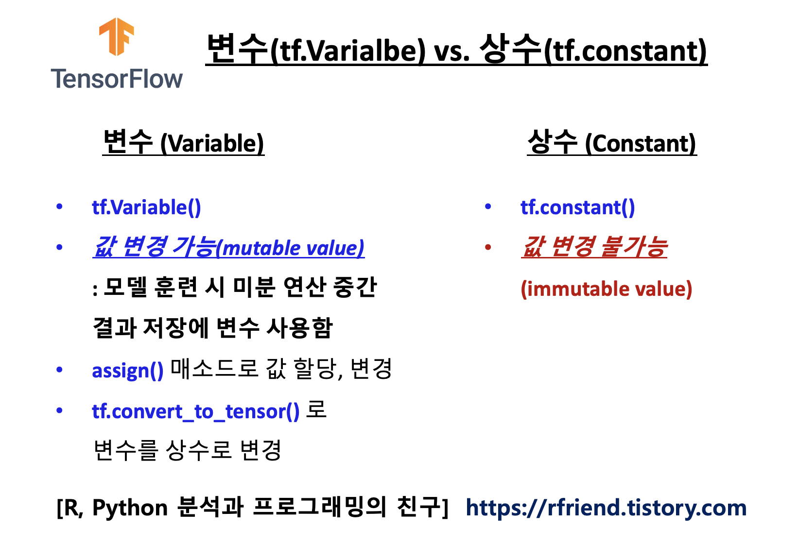
 텐서플로의 튜토리얼의 소개를 보면 "변수는 프로그램 연산에서 공유되고 유지되는 상태를 표현하는데 사용을 권장("A TensorFlow variable is the recommended way to represent shared, persistent state your program manipulates.") 한다고 합니다. 말이 좀 어려운데요, 변수와 상수를 비교해보면 금방 이해가 갈 것입니다. 

 텐서플로 변수(Variable)는 값의 변경이 가능(mutable value)한 반면에, 상수(constant)는 값의 변경이 불가능(immutable value)합니다. 변수는 값의 변경이 가능하고 공유되고 유지되는 특성 때문에 딥러닝 모델을 훈련할 때 자동 미분 값의 back-propagations 에서 가중치를 업데이트한 값을 저장하는데 사용이 됩니다. 변수는 초기화(initialization)가 필요합니다. 

(2) TensorFlow 변수를 만들고(tf.Variable), 값을 변경하는 방법 (assign)

TensorFlow 변수는 tf.Variable(value, name, dtype, shape) 의 메소드를 사용해서 만들 수 있습니다. 

import tensorflow as tf
print(tf.__version__)
#2.7.0


## After construction, the type and shape of the variable are fixed.
v = tf.Variable([1, 2])
print(v)
#<tf.Variable 'Variable:0' shape=(2,) dtype=int32, numpy=array([1, 2], dtype=int32)>

변수의 값을 변경할 때는 assign() 메소드를 사용합니다.  assign_add(), assign_sub() 를 사용해서 덧셈이나 뺄셈 연산을 수행한 후의 결과로 변수의 값을 업데이트 할 수도 있습니다. 

## The value can be changed using one of the assign methods.
v.assign([3, 4])

print(v)
#<tf.Variable 'Variable:0' shape=(2,) dtype=int32, numpy=array([3, 4], dtype=int32)>


## The value can be changed using one of the assign methods.
v.assign_add([10, 20])

print(v)
#<tf.Variable 'Variable:0' shape=(2,) dtype=int32, numpy=array([13, 24], dtype=int32)>

tf.Variable(value, shape=tf.TensorShape(None)) 처럼 shape 매개변수를 사용하면 형태(shape)를 정의하지 않은 상태에서 변수를 정의할 수도 있습니다. 

## The shape argument to Variable's constructor allows you to 
## construct a variable with a less defined shape than its initial-value
v = tf.Variable(1., shape=tf.TensorShape(None))

print(v)
#<tf.Variable 'Variable:0' shape=<unknown> dtype=float32, numpy=1.0>


v.assign([[1.]])
#<tf.Variable 'UnreadVariable' shape=<unknown> dtype=float32, 
#numpy=array([[1.]], dtype=float32)>

(3) TensorFlow 변수 연산 (operations)

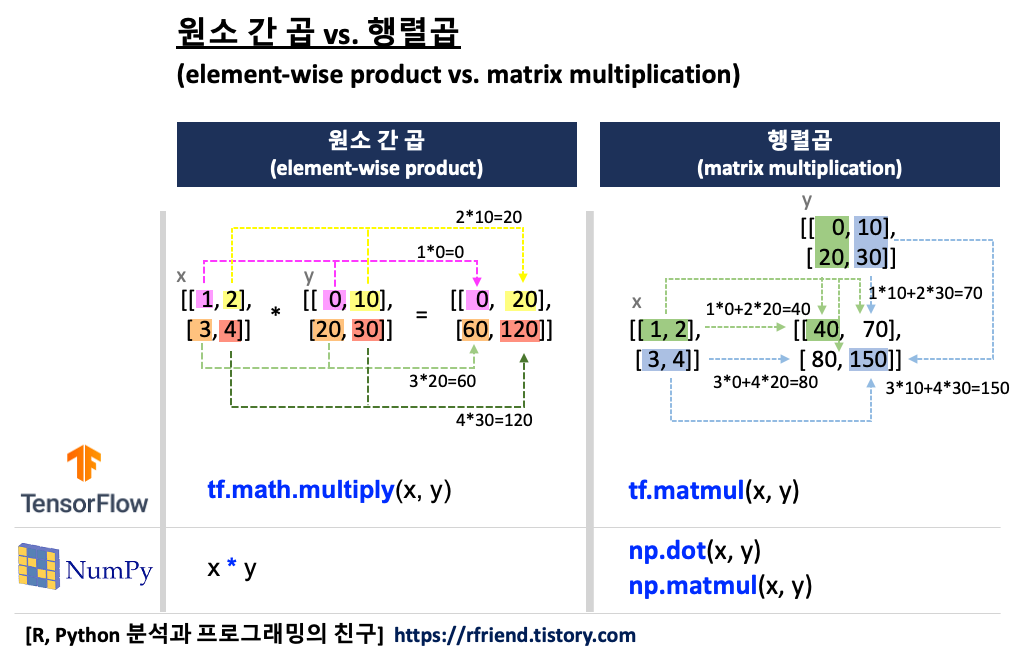
변수는 텐서 연산의 인풋(inputs to operations)으로 사용될 수 있습니다. 아래 예에서는 변수와 상수간 원소 간 곱과 합을 구해보았습니다. 

## Variable created with Variable() can be used as inputs to operations. 
## Additionally, all the operators overloaded for the Tensor class are carried over to variables. 
w = tf.Variable([1., 2.])
x = tf.constant([3., 4.])

## element-wise product
tf.math.multiply(w, x)
# <tf.Tensor: shape=(2,), dtype=float32, numpy=array([3., 8.], dtype=float32)>



## element-wise addition
w + x
# <tf.Tensor: shape=(2,), dtype=float32, numpy=array([4., 6.], dtype=float32)>

(4) TensorFlow 변수 속성 정보 (attributes)

텐서플로의 변수에서 이름(name), 형태(shape), 데이터 유형(dtype), 연산에 이용되는 디바이스(device) 속성정보를 조회할 수 있습니다. 

## Attributes
v = tf.Variable([1., 2.], name='MyTensor')
print('name:', v.name)
print('shape:', v.shape)
print('dtype:', v.dtype)
print('device:', v.device)

# name: MyTensor:0
# shape: (2,)
# dtype: <dtype: 'float32'>
# device: /job:localhost/replica:0/task:0/device:CPU:0

(5) 변수를 상수로 변환하기 (converting tf.Variable to tf.constant)

변수를 상수로 변환하려면 tf.convert_to_tensor(Variable) 메소드를 사용합니다. 

## converting tf.Variable to Tensor
c = tf.convert_to_tensor(v)

print(c)
# tf.Tensor([1. 2.], shape=(2,), dtype=float32)

[ Reference ]

* TensorFlow Variable: https://www.tensorflow.org/api_docs/python/tf/Variable

이번 포스팅이 많은 도움이 되었기를 바랍니다 

행복한 데이터 과학자 되세요!  :-)

데이터 전처리를 하다보면 필요에 맞게 데이터 형태, 구조를 변경하는 일이 빈번하게 생깁니다. 이번 포스팅에서는 텐서의 형태를 변환, 재구조화, 전치하는 방법을 소개하겠습니다. 

이미 numpy (https://rfriend.tistory.com/345 , https://rfriend.tistory.com/289)에 익숙한 분이라면, 사용법이 비슷하기 때문에 그리 어렵지 않게 금방 이해할 수 있을 거예요. 

(1) tf.reshape(): 텐서의 형태 변환 

(2) tf.transpose(): 텐서의 행과 열 전치

(1) tf.reshape(): 텐서의 형태 변환

먼저, 0~11까지 12개의 원소를 가지는 벡터(vector) 로 텐서를 만들어보겠습니다. 

t1 = tf.constant(range(12))

print(t1)
# tf.Tensor([ 0  1  2  3  4  5  6  7  8  9 10 11], 
#.          shape=(12,), dtype=int32)


tf.rank(t1) # rank 1
# <tf.Tensor: shape=(), dtype=int32, numpy=1>

위의 벡터 (12,) 형태를 가지는 텐서 t1을, 행렬 (3, 4) 형태를 가지는 텐서로 tf.reshape(tensor, shape, name=None) 메소드를 사용해서 변환(reshape)해보겠습니다. 

## reshaping a shape of Tensor from (12,) to (3, 4)
t2 = tf.reshape(t1, [3, 4]) 

print(t2)
# tf.Tensor(
# [[ 0  1  2  3]
#  [ 4  5  6  7]
#  [ 8  9 10 11]], shape=(3, 4), dtype=int32)


tf.rank(t2) # rank 2
# <tf.Tensor: shape=(), dtype=int32, numpy=2>

tf.reshape(tensor, shape) 의 shape 란에 원하는 형태를 [ ] 안에 콤마로 구분해서 넣어주면 됩니다. 이번에는 rank 3 을 가지는 (2, 2, 3) 형태의 텐서로 형태를 변환해보겠습니다. 

## reshaping a Tensor with a shape of (12,) to (2,2,3)
t3 = tf.reshape(t1, [2, 2, 3])

print(t3)
# tf.Tensor(
# [[[ 0  1  2]
#   [ 3  4  5]]
#  [[ 6  7  8]
#   [ 9 10 11]]], shape=(2, 2, 3), dtype=int32)


tf.rank(t3) # rank 3
# <tf.Tensor: shape=(), dtype=int32, numpy=3>

tf.reshape(tensor, shape) 의 shape 에 '-1' 이 들어있으면, 숫자가 기입된 부분의 축을 변환하고 난 후에, "남은 축의 형태는 원래 텐서의 총 크기와 같도록 알아서 추정"해준다는 뜻입니다. 

아래 예에서는 원래 텐서 t1 이 (12,) 형태였으며, tf.reshape(t1, [-1, 3]) 으로 재구조화시켰더니 (4, 3) 형태의 텐서로 변환되었네요. 

## If one component of shape is the special value -1, 
## the size of that dimension is computed 
## so that the total size remains constant.
t4 = tf.reshape(t1, [-1, 3])


print(t4)
# tf.Tensor(
# [[ 0  1  2]
#  [ 3  4  5]
#  [ 6  7  8]
#  [ 9 10 11]], shape=(4, 3), dtype=int32)


tf.rank(t4) # rank 2
# <tf.Tensor: shape=(), dtype=int32, numpy=2>

특히, tf.reshape(tensor, [-1]) 처럼 shape 에 [-1] 은 1차원의 벡터인 1-D 텐서로 변환을 한다는 뜻입니다. 

아래 예에서 텐서 t4 는 (4, 3) 형태를 가지는 행렬이었는데요, tf.reshape(t4, [-1]) 해주었더니 (12,) 의 형태를 가지는 1차원의 벡터로 변환이 되었습니다. 

## In particular, a shape of [-1] flattens into 1-D. 
## At most one component of shape can be -1.
t5 = tf.reshape(t4, [-1])

print(t5)
# tf.Tensor([ 0  1  2  3  4  5  6  7  8  9 10 11], 
#           shape=(12,), dtype=int32)


tf.rank(t5) # rank 1
# <tf.Tensor: shape=(), dtype=int32, numpy=1>

tf.reshape(tensor, []) 의 [ ] 는 텐서를 1개의 원소를 가지는 스칼라(scalar) 로 변환합니다. 

## tf.reshape(t, []) reshapes a tensor t with one element to a scalar.
t6 = tf.constant([5])

print(t6) # rank 1, vector
# tf.Tensor([5], shape=(1,), dtype=int32)


t7 = tf.reshape(t6, [])
print(t7) # rank 0, scalar
# tf.Tensor(5, shape=(), dtype=int32)


tf.rank(t7) # rank 0
# <tf.Tensor: shape=(), dtype=int32, numpy=0>

(2) tf.transpose(): 텐서의 행과 열 전치

tf.transpose(tensor)는 텐서의 행과 열의 위치를 전치(transpose) 시켜 줍니다. 

아래의 예에서는 shape=(3,4) 의 텐서를 shape=(4,3)의 텐서로 행과 열을 전치시켜주었습니다. 행과 열이 전치를 시키기 전과 후에 어떻게 바뀌었는지 살펴보면 금방 이해하실 수 있을 거예요. 

print(t2)
# tf.Tensor(
# [[ 0  1  2  3]
#  [ 4  5  6  7]
#  [ 8  9 10 11]], shape=(3, 4), dtype=int32)


t8 = tf.transpose(t2)

print(t8)
# tf.Tensor(
# [[ 0  4  8]
#  [ 1  5  9]
#  [ 2  6 10]
#  [ 3  7 11]], shape=(4, 3), dtype=int32)

[ Reference ]

- tf.reshape(): https://www.tensorflow.org/api_docs/python/tf/reshape

- tf.transpose(): https://www.tensorflow.org/api_docs/python/tf/transpose

이번 포스팅이 많은 도움이 되었기를 바랍니다. 

행복한 데이터 과학자 되세요!  :-)

딥러닝 모델을 훈련하고 예측하는데 사용하는 TensorFlow 프레임웍의 이름은 Tensor + Flow (텐서를 흘려보냄) 에서 유래했습니다. 텐서(Tensor)는 텐서플로의 가장 기본이 되는 자료 구조인 만큼 만드는 방법과 속성정보 조회하는 방법을 알아둘 필요가 있겠습니다. 

이번 포스팅에서는 

(1) 텐서의 정의

(2) 텐서 만들기

     - (2-1) tf.constant([mat1, mat2, mat3])

     - (2-2) tf.stack([mat1, mat2, mat3])

     - (2-3) tf.convert_to_tensor([mat1, mat2, mat3])

(3) 텐서의 속성정보 조회하기

     - (3-1) Tensor.dtype : 텐서 데이터 유형

     - (3-2) Tensor.shape : 텐서 형태

     - (3-3) Tensor.rank : 텐서 차수(rank), 텐서를 구성하는 벡터의 개수, 랭크

     - (3-4) Tensor.device : 텐서 생성 디바이스 (CPU, GPU)

하는 방법에 대해서 소개하겠습니다. 

(1) 텐서의 정의

 TensorFlow의 자료 구조에는 0차원의 스칼라(scalar), 1차원의 벡터(vector), 2차원의 행렬(matrix), 3차원 이상의 텐서(tensor) 가 있습니다. 텐서플로에서 텐서는 벡터와 행렬, 그리고 3차원 이상의 고차원의 배열을 모두 아우르는 일반화된 데이터 구조를 말합니다.

 텐서플로는 파이썬 객체를 텐서(Tensor)로 변환해서 행렬 연산을 수행합니다. 텐서플로는 먼저 tf.Tensor 객체의 그래프(graph) 를 생성하는 것에서 시작하여, 각 텐서가 어떻게 계산되는지를 구체화하고, 이 그래프의 부분들을 실행하여 원하는 최종 결과를 도출합니다. 

 텐서는 데이터 유형(a data type, 예: float32, int32, string) 과 데이터 형태 (shape) 의 속성을 가집니다. 

(2) 텐서 만들기

그럼, (2, 3) 의 shape 을 가지는 3개의 배열을 가지고, 3차원인 (3, 2, 3) 형태의 텐서를 만들어보겠습니다. 

     - (2-1) tf.constant([mat1, mat2, mat3])

     - (2-2) tf.stack([mat1, mat2, mat3])

     - (2-3) tf.convert_to_tensor([mat1, mat2, mat3])

import tensorflow as tf
tf.__version__
#2.7.0


## input matrix (list of list)
mat1 = [[1, 2, 3], [4, 5,  6]]
mat2 = [[7, 8, 9], [10, 11, 12]]
mat3 = [[13, 14, 15], [16, 17, 18]]

(2-1) tf.constant([mat1, mat2, mat3])

## A tf.Tensor represents a multidimensional array of elements.

## (1) tf.constant(): Creates a constant tensor from a tensor-like object.
tensor1 = tf.constant([mat1, mat2, mat3])

tensor1
# <tf.Tensor: shape=(3, 2, 3), dtype=int32, numpy=
# array([[[ 1,  2,  3],
#         [ 4,  5,  6]],

#        [[ 7,  8,  9],
#         [10, 11, 12]],

#        [[13, 14, 15],
#         [16, 17, 18]]], dtype=int32)>

(2-2) tf.stack([mat1, mat2, mat3])

## tf.stack(): Stacks a list of rank-R tensors into one rank-(R+1) tensor.
tensor2 = tf.stack([mat1, mat2, mat3])

(2-3) tf.convert_to_tensor([mat1, mat2, mat3])

텐서를 만들 때 데이터 유형(dtype), 텐서 이름(name)의 속성정보를 설정할 수 있습니다. 

## tf.convert_to_tensor(): Converts the given value to a Tensor.
tensor3 = tf.convert_to_tensor([mat1, mat2, mat3])

# tensor3 = tf.convert_to_tensor([mat1, mat2, mat3], 
#                                dtype=tf.int64, 
#                                name='my_first_tensor')

(3) 텐서의 속성정보 조회하기

     - (3-1) Tensor.dtype : 텐서 데이터 유형

     - (3-2) Tensor.shape : 텐서 형태

     - (3-3) Tensor.rank : 텐서 차수(rank), 텐서를 구성하는 벡터의 개수, 랭크

     - (3-4) Tensor.device : 텐서 생성 디바이스 (CPU, GPU)

# A tf.Tensor has the following properties:
# - a single data type (float32, int32, or string, for example)
# - a shape

## The DType of elements in this tensor.
tensor3.dtype
# tf.int64


## Returns a tf.TensorShape that represents the shape of this tensor.
tensor3.shape
# TensorShape([3, 2, 3])


## rank of this tensor.
tf.rank(tensor3)
# <tf.Tensor: shape=(), dtype=int32, numpy=3>


## The name of the device on which this tensor will be produced, or None.
tensor3.device
# /job:localhost/replica:0/task:0/device:GPU:0

[ Referece ]

- tf.Tensor(): https://www.tensorflow.org/api_docs/python/tf/Tensor

- tf.constant(): https://www.tensorflow.org/api_docs/python/tf/constant

- tf.stack(): https://www.tensorflow.org/api_docs/python/tf/stack

- tf.convert_to_tensor(): https://www.tensorflow.org/api_docs/python/tf/convert_to_tensor

이번 포스팅이 많은 도움이 되었기를 바랍니다. 

행복한 데이터 과학자 되세요!  :-)

이번 포스팅에서는 Python Tensorflow와 numpy 모듈을 사용하여 

  (1) 행렬 원소 간 곱 (matrix element-wise product)

  (2) 행렬 곱 (matrix multiplication) 

하는 방법과 연산 방법을 소개하겠습니다. 

얼핏보면 둘이 비슷해보이지만, 전혀 다른 연산으로서 주의가 필요합니다. 

먼저, TensorFlow와 numpy  모듈을 불러오고, 예제로 사용할 2차원 행렬(matrix)을 만들어보겠습니다. 

import numpy as np
import tensorflow as tf
print(tf.__version__)
#2.7.0


## matrix
x = tf.constant([[1, 2], [3, 4]])

print(x)
# tf.Tensor(
# [[1 2]
#  [3 4]], shape=(2, 2), dtype=int32)


y = tf.constant([[0, 10], [20, 30]])

print(y)
# tf.Tensor(
# [[ 0 10]
#  [20 30]], shape=(2, 2), dtype=int32)

(1) 행렬 원소 간 곱 (matrix element-wise product)

## [TensorFlow] matrix element-wise product
tf.math.multiply(x, y)

# <tf.Tensor: shape=(2, 2), dtype=int32, numpy=
# array([[  0,  20],
#        [ 60, 120]], dtype=int32)>

## [numpy] matrix element-wise produce
np.array(x) * np.array(y)

# array([[  0,  20],
#        [ 60, 120]], dtype=int32)

(2) 행렬 곱 (matrix multiplication) 

## matrix multiplication using tf.matmul()
tf.matmul(x, y)

# <tf.Tensor: shape=(2, 2), dtype=int32, numpy=
# array([[ 40,  70],
#        [ 80, 150]], dtype=int32)>

## [numpy] matrix multiplication using np.dot()
np.dot(x, y)

# array([[ 40,  70],
#        [ 80, 150]], dtype=int32)



## [numpy] matrix multiplication using np.matmul()
np.matmul(x, y)

# array([[ 40,  70],
#        [ 80, 150]], dtype=int32)

참고로, TensorFlow 의 텐서를 numpy의 array 로 변환하려면 numpy() 메소드를 사용하면 됩니다. 

## casting tensor to numpy's array
tf.matmul(x, y).numpy()

# array([[ 40,  70],
#        [ 80, 150]], dtype=int32)

이번 포스팅이 많은 도움이 되었기를 바랍니다. 

행복한 데이터 과학자 되세요!  :-)

"Colab" 은 Google Colaboratory 를 줄여서 쓴 것으로, Google Research 팀에서 개발한 서비스 제품입니다. Colab을 사용하면 웹브라우저를 통해서 클라우드 상에서 CPU뿐만 아니라 GPU나 TPU도 무료로(!!!) 사용하여 Python과 Jupyter Notebook으로 데이터 분석을 할 수 있습니다. 

물론 무료로 Colab을 이용하려면 Resource 한도가 있기는 합니다만, 교육용이나 간단한 실습용으로 GPU 또는 TPU를 써서 기계학습 모델을 훈련시켜보기에는 손색이 없습니다. 

Colab 한도를 높여서 더 빠른 GPU, 더 긴 타임, 추가 메모리를 사용하고 싶으면 $9.99/월 유료 Colab Pro 를 이용하면 됩니다. (무료는 최대 12시간 vs. Colab Pro는 최대 24시간) 

이번 포스팅에서는 Google Colab에서 외부 데이터를 로딩해서 이용할 수 있는 2가지 방법을 소개하겠습니다. 

(1) Local folder에서 Colab 으로 파일 로딩하기 

    (Loading a file from the local folder to Colab)

(2) Google Drive를 Colab에 연결해서 데이터 로딩하기 

    (Mounting google drive to Colab) (추천)

Google Colab을 시작하려면, 먼저 Google Drive에 접속한 후에 왼쪽 상단의 '+ New' 메뉴를 선택한 후, 

'More' 메뉴의 오른쪽 꺽쇠 화살표를 눌러 나온 추가 메뉴에서 'Google Colaboratory' 를 선택해주면 됩니다. 

그러면 아래처럼 Colab Jupyter Notebook 이 론칭됩니다. (backend 에서 도커 이미지 생성되어 돌아가고 있음.)

CPU, GPU, 또는 TPU 를 사용할지 여부는 Runtime > Change runtime type 메뉴에서 선택할 수 있습니다.

만약 Colab에서 로컬 머신에 있는 폴더 내 파일을 읽어오려고 하면 "FileNotFoundError: [Errno 2] No such file or directory: your_local_path_here" 라는 에러 메시지가 나올 겁니다. Google 의 클라우드에서 작동하고 있는 Colab 은 로컬 머신의 경로를 인식하지 못하기 때문에 이런 에러가 발생합니다.("우물가에서 숭늉 찾는 격"이라고 할까요...)  

이럴 때 필요한게 Local machine 의 folder에서 파일을 Colab으로 로딩해서 사용하는 방법입니다. Google Colab에서 쉽게 로컬 폴더에서 업로드할 수 있도록 해주는 메소드인 google.colab.files.upload() 를 제공합니다. 

Colab에서 아래처럼 코드를 실행하면 '파일 선택' 하는 메뉴가 나타납니다. 

'파일 선택' 메뉴를 선택하면 아래와 같이 '탐색기 창'이 팝업으로 나타납니다. 원하는 위치에서 원하는 파일을 선택한 후 '열기' 메뉴를 선택해줍니다. 

선택한 'abalone.txt' 파일이 Colab 으로 업로딩이 완료되면 아래 화면캡쳐처럼 '100% done' 이라는 메시지와 함께 'Saving abalone.txt to abalone.txt' 라는 안내 메시지가 뜹니다. 

위에서 업로딩한 'abalone.txt' 텍스트 파일을 읽어와서 Pandas DataFrame으로 만들어보겠습니다. 이때 pd.read_csv()를 바로 사용하면 안되며, Python으로 다양한 I/O 스트림을 다룰 때 사용하는 io 모듈을 사용해서 io.BytesIO(file_uploaded['abalone.txt'] 로 '_io.BytesIO object'를 먼저 만들어준 다음에 pandas.read_csv() 메소드로 Pandas DataFrame을 만들 수 있습니다. 

그런데, 이 방법은 로컬 머신에 수동으로 경로를 찾아가서 하나씩 파일 열기를 하여 읽어와야 하는 번거로움이 있고, 구글 드라이브 클라우드 내에서 모든 걸 해결할 수 있는 더 편리하고 폴더 채 데이터에 접근할 수 있는 더 강력한 방법이 있습니다. 그게 다음에 설명할 Google Drive를 Colab에 연결(mounting)해서 사용하는 방법입니다. 

Google Drive를 Colab에 올려서(mounting) 사용하는 방법이 전에는 인증, API 연결같은게 좀 까탈스러웠는데요, 지금은 아래처럼 google.colab.drive.mount('/content/drive') 를 해주고 'authorization code' 만 복사해서 넣어주면 되게끔 깔끔하게 간소화되었습니다. 

아래 화면캡쳐에서 'Go to this URL in a browser: https://xxxx ' 부분의 URL 링크를 클릭해줍니다. 

그러면 아래 화면처럼 'Sign in with Google' 팝업 창의 'Choose an account to continue to Google Drive File Stream' 에서 데이터가 들어있는 자신의 구글 계정을 선택해서 클릭해줍니다. 

다음으로, 아래 화면캡쳐처럼 'Google Drive File Stream에서 내 Google 계정에 액세스하려고 합니다.' 안내창이 뜨면 하단의 '허용'을 선택해줍니다. 

이제 거의 다 왔네요. 아래 화면캡쳐처럼 'Google 로그인: 이 코드를 복사하여 애플리케이션으로 전환한 다음 붙여넣으세요' 라는 메시지가 뜨는데요, '인증 코드를 복사'합니다. 

바로 위에서 복사한 '인증코드'를 Google Colab Jupyter Notebook으로 다시 돌아와서 아래의 'Enter your authorization code:' 의 아래 빈 칸에 붙여넣기를 해주고 Jupyter notebook cell 을 실행시킵니다. 

자, 이제 Google Drive를 Colab 위에 올려놓기(mounting)를 성공했으므로 Colab의 왼쪽 상단의 '폴더' 아이콘을 클릭하여 탐색기 모드로 전환하고 폴더와 파일을 찾아봅시다.  저기에 Google Drive에 올라가 있는 'abalone.txt' 파일이 보이는군요. 이 파일의 오른쪽 끝에 ':' 을 클릭한 후 'Copy path'를 선택해서 'abalone.txt' 파일이 있는 경로를 복사해놓습니다. 

바로 위에서 'Copy path'로 복사한 'abalone.txt' 파일이 있는 경로(path)를 붙여넣기 해서 보니 '/content/abalone.txt' 입니다. 이 경로를 pd.read_csv() 에 바로 입력해서 pandas DataFrame 으로 만들어보겠습니다. 

참고로, 위에서 처럼 마우스로 폴더 탐색기 눌러서 하나씩 찾아가는 방법 말고, Python의 os 모듈을 이용하면 Colab의 현재 작업경로(os.getcwd(), current working directory), 폴더와 파일 리스트 (os.listdir()), 경로에 특정 파일이 존재하는지 여부(os.path.isfile()) 등을 편리하게 확인할 수 있습니다. 

만약에 여러개의 파일들을 폴더별로 계층적으로 정리하여 놓은 데이터를 이용해야 하는 경우라면 아래처럼 Google Drive에 로컬에 있는 폴더를 통째로 올려서 사용할 수도 있습니다. 

저는 로컬 머신의 다운로드 폴더에 들어있는 'dogs_cats_sample' 폴더를 통째로 Google Drive에 업로드해보겠습니다. 'dogs_cats_sample' 폴더 밑에는 'output', 'test', 'train', 'validation' 하위 폴더가 있으며, 이들 각 폴더에는 개와 고양이 이미지 jpg 파일들과 정답 라벨 텍스트 파일이 들어있습니다. 폴더를 통째로 Google Drive 에 한번에 올릴 수 있어서 정말 편리합니다. 

개와 고양이 jpg 이미지들과 라벨 데이터가 Google Drive에 업로드가 되는데 시간이 좀 걸립니다. 업로드가 완료되면 아래 화면처럼 Colab의 왼쪽 사이드바에서 '폴더' 모양 아이콘을 클릭하여 보조창을 열고, 'drive > My Drive > 0_dogs_cats_sample' 폴더를 찾아가서 선택한 후 'Copy path'를 클릭하면 '0_dogs_cats_sample' 폴더의 경로를 복사할 수 있습니다. 

위에서 복사한 경로를 붙여넣기 해서 보면 '/content/drive/My Drive/0_dogs_cats_sample' 경로에 잘 업로드되어 있음을 알 수 있습니다. 아래에는 이들 폴더 내 이미지 파일들 중에서 'train/cat/cat.1.jpg' 이미지 파일 하나를 가져와서 시각화해보았습니다. 

[ Reference ]

* Coalbroatory FAQs: https://research.google.com/colaboratory/faq.html

* How to mount Google drive to Colab: https://colab.research.google.com/notebooks/io.ipynb#scrollTo=u22w3BFiOveA

* Python io module: https://docs.python.org/3/library/io.html

많은 도움이 되었기를 바랍니다. 

이 포스팅이 도움이 되었다면 아래의 '공감~'를 꾹 눌러주세요. 

희소행렬(Sparse matrix)은 대부분의 값이 원소 '0'인 행렬, '0'이 아닌 원소가 희소(sparse)하게, 듬성듬성 있는 행렬을 말합니다. 반대로 밀집행렬(Dense matrix)은 대부분의 원소 값이 '0'이 아닌 행렬을 말합니다. 

자연어처리 분석을 할 때 문서 내 텍스트를 컴퓨터가 이해할 수 있는 형태의 자료구조로 만들 때 텍스트 파싱을 거쳐 단어-문서 행렬(Term-Document matrix) (or 문서-단어 행렬, Document-Term matrix) 를 만드는 것부터 시작합니다. 

문서별로 많은 수의 단어가 포함되어 있고, 또 단어별로 발생 빈도가 보통은 드물기 때문에, 문서에서 단어를 파싱하여 Term-Document 행렬을 만들면 대부분은 희소행렬(Sparse matrix)을 얻게 됩니다. 

이번 포스팅에서는 

(1) 문서별 단어로 부터 CSR 행렬(Compressed Sparse Row matrix) 을 만들고, 

(2) CSR 행렬을 이용해 NumPy array의 Term-Document 행렬 만들기

를 해보겠습니다. 

단, 이번 포스팅의 주 목적은 문서로부터 문서-단어 CSR 행렬을 만들고 --> 이를 NumPy array의 Term-Document 행렬을 만드는 과정에 집중해서 소개하는 것으로서, 텍스트 파싱하는데 필요한 세부 절차(가령 문장 분리, 대문자의 소문자로 변환, Stop words 생략 등)는 생략합니다. 

(텍스트를 단어 단위로 파싱해서 one-hot encoding 하는 방법은 https://rfriend.tistory.com/444 포스팅 참조하세요.)

먼저, NumPy와 SciPy 모듈을 importing 하겠습니다. 

아래와 같이 리스트 [] 하나를 문서(Document) 하나로 간주했을 때, 총 3개의 문서를 가진 "docs" 로 부터 단어(Term)를 파싱해서 단어집(Vocabulary) 사전형(dictionary)을 만들고, 압축 희소 행기준 행렬(Compressed Sparse Row matrix) 을 만들기 위해 필요한 indptr, indices, data 객체를 for loop 문을 써서 만들어보겠습니다. 

참고로, CSR 행렬 소개, SciPy.sparse.csr_matrix() 메소드 소개, NumPy 희소행렬을 SciPy 압축 희소 행기준 행렬 (Compressed Sparse Row matrix) 로 변환하는 방법은 https://rfriend.tistory.com/551 포스팅을 참고하세요. 

* reference: https://docs.scipy.org/doc/scipy/reference/generated/scipy.sparse.csr_matrix.html

위의 실행결과로 얻은 단어집(Vocabulary)을 Key : Value 쌍으로 출력을 해서 살펴보겠습니다. 3개의 문서에 총 7개의 단어가 있군요. (문서별로 중복되는 단어(term)가 존재함)

[Out]

python : 0
is : 1
a : 2
programming : 3
language : 4
fun : 5
easy : 6

위에서 얻은 indptr, indices, data 를 가지고 SciPy.sparse.csr_matrix() 메소드를 이용하여 압축 희소 행기준 행렬(CSR matrix)을 만들어보겠습니다.  

[Out] <3x7 sparse matrix of type '<class 'numpy.int64'>'
	with 11 stored elements in Compressed Sparse Row format>

[Out]

  (0, 0)	1
  (0, 1)	1
  (0, 2)	1
  (0, 3)	1
  (0, 4)	1
  (1, 3)	1
  (1, 1)	1
  (1, 5)	1
  (2, 0)	1
  (2, 1)	1
  (2, 6)	1

-- SciPy Compressed Sparse Row matrix --
indptr: [ 0  5  8 11]
indices: [0 1 2 3 4 3 1 5 0 1 6]
data: [1 1 1 1 1 1 1 1 1 1 1]

위의 (1)번에서 만든 SciPy CSR(Compressed Sparse Row) matrix를 csr_matrix.toarray() 또는 csr_matrix.todense() 메소드를 사용해서 NumPy array 행렬로 변환해보겠습니다. 이로부터 Term-Document Matrix를 만들었습니다. 

[Out]

array([[1, 1, 1, 1, 1, 0, 0],
       [0, 1, 0, 1, 0, 1, 0],
       [1, 1, 0, 0, 0, 0, 1]])

많은 도움이 되었기를 바랍니다. 

이번 포스팅이 도움이 되었다면 아래의 '공감~'를 꾹 눌러주세요. 

이번 포스팅에서는 파일 형태의 이미지 데이터를 TensorFlow와 Keras 메소드를 사용하여

(1) 웹에서 압축 이미지 파일을 다운로드하여 압축을 해제하고,

(2) 폴더 이름을 확인하고 폴더 밑에 있는 파일 이름을 리스트로 만들기

(3) 이미지 파일을 로딩하여 시각화하고 라벨 이름 출력하기

를 해보겠습니다.

먼저 TensorFlow 와 객체지향 파일시스템 경로(object-oriented filesystem paths)를 관리할 때 사용하는 pathlib 모듈을 importing 하겠습니다.

[Out] 2.4.0-dev20200913

이제 준비가 되었으니 https://storage.googleapis.com 의 예제 이미지로 압축되어 저장되어 있는 'flower_photos.tgz' 압축 파일을 Keras의 get_file() 메소드를 사용하여 가져와서 압축을 풀어(untar = True)보겠습니다.

이러면 압축이 풀린 파일이 '.keras/datasets/flower_photos 라는 폴더에 저장되어 있습니다. 이를 pathlib.Path() 메소드로 Mac, Linux, Windows OS에 상관없이 경로를 인식할 수 있도록 PurePath로 만들어주었습니다.

* source: https://docs.python.org/3/library/pathlib.html

[Out] /Users/xxx/.keras/datasets/flower_photos

[Out] PosixPath('/Users/xxx/.keras/datasets/flower_photos')

저는 Mac OS 에서 작업을 했는데요, Mac OS에서 숨겨진 폴더, 파일을 보려면 Finder 에 커서를 가져다대고 'Shift + Command + .' 을 동시에 눌러주면 됩니다. 그러면 아래의 화면 캡쳐처럼 '/.keras/datasets/flower_photos/' 경로에 다운로드 후 압축해제한 이미지 파일들이 들어있음을 눈으로 직접 확인할 수 있습니다.

다음으로, root directory 밑에 있는 하위 디렉토리와 파일 이름들을 모두(flowers_root.glob("*") ) 가져다가 for loop 으로 순회하면서 하나씩 차례대로 출력해서 확인해보겠습니다.

위의 화면캡쳐에서 숨겨진 폴더, 파일을 눈으로 봤던 것과 동일하게 하위 폴더에는 'roses', 'sunflowers', 'daisy', 'dandelion', 'tulips' 폴더와 'LICENSE.txt' 텍스트 파일이 들어있군요.

[Out]
roses
sunflowers
daisy
dandelion
tulips
LICENSE.txt

이제 TensorFlow.Dataset.list_files() 메소드를 사용해서 각 꽃 이름 폴더 ('roses', 'sunflowers', 'daisy', 'dandelion', 'tulips' 폴더) 밑에 있는 이미지 파일 이름(jpg 포맷) 들의 리스트를 만들어보겠습니다.

그리고 이중에서 3개만 가져와서(take(3)) 하나씩 차례대로 '전체 경로/파일이름'을 출력해보겠습니다.

b'/Users/xxx/.keras/datasets/flower_photos/daisy/4440480869_632ce6aff3_n.jpg'
b'/Users/xxx/.keras/datasets/flower_photos/daisy/1879567877_8ed2a5faa7_n.jpg'
b'/Users/xxx/.keras/datasets/flower_photos/sunflowers/969913643_9d5cd2fe45_m.jpg'

이제 이미지 파일이 준비가 되었으니 TensorFlow.keras.preprocessing.image 메소드를사용하여 꽃 이미지 3개를 크기가 (250, 250)인 이미지로 변환하여 로딩하고, matplotlib 모듈로 시각화(plt.imshow(img))해보겠습니다. ( tf.Tensor() 파일을 f.numpy() 로 변환하여 로딩)

이때 TensorFlow.strings.split(f, os.sep)[-2] 로 '전체 경로/파일이름' 리스트에서 뒤에서 부터 두번째에 위치한 라벨을 파싱해서 가져와서 이미지를 시각화할 때 라벨도 같이 출력을 해보겠습니다.

해바라기(sunflowers), 장미(roses), 민들레(dandelions) 이 차례대로 시각화되었네요.

* Reference: https://www.tensorflow.org/guide/data?hl=en

많은 도움이 되었기를 바랍니다.

이번 포스팅이 도움이 되었다면 아래의 '공감~'를 꾹 눌러주세요.

자동미분(Automatic differentiation, Algorithmic differentiation, computational differentiation, auto-differentiation, 또는 줄여서 간단히 auto-diff) 은 컴퓨터 프로그램에 의해서 구체화된 함수의 미분을 산술적으로 계산할 때 사용하는 기술의 집합을 말합니다. 컴퓨터 프로그램에서 구체화한 함수는 아무리 복잡해보이더라도 기본적인 산술 연산 (덧셈, 뺄셈, 곱셉, 나눗셈 등)과 기본적인 함수 (지수, 로그, 싸인, 코싸인 등) 의 연속적인 실행으로 이루어진다는 아이디어를 기반으로 합니다. 복잡한 함수도 연쇄 법칙(Chain Rule)을 이용함으로써 합성함수를 구성하는 각 기본함수의 미분의 곱으로 나타내고 반복적으로 계산함으로써 자동으로 복잡한 함수를 정확하고 효율적으로 미분할 수 있습니다.   

자동미분(Automatic Differentiation)은 딥러닝에서 오차 역전파 알고리즘을 사용해서 모델을 학습할 때 유용하게 사용합니다. TensorFlow는 Gradient Tapes 를 이용하면 즉시 실행 모드(eager execution mode)에서 쉽게 오차 역전파를 수행할 수 있습니다. 

이번 포스팅에서는 

1. 즉시실행모드에서 자동미분을 하기 위해 Gradient tapes 이 필요한 이유

2. TensorFlow에서 Gradient tapes를 이용해 자동미분하는 방법

3. 시그모이드 함수 자동미분 시각화

4. 테이프가 볼 것을 조정하는 방법 (Controlling what the tape watches)

5. Python 조건절 분기문을 이용한 테이프 기록 흐름 조정 (Control flow)

에 대해서 소개하겠습니다. 

이번 포스팅은 TensorFlow 튜토리얼의 내용을 번역하고 코드를 대부분 사용하였습니다. 

먼저 numpy, tensorflow, matplotlib 모듈을 importing 하겠습니다. 

2.4.0-dev20200913

예를 들어서  y = a * x 라는 방정식에서 a 와 y 가 상수(constant)이고 x 가 변수(Varialbe) 일 때, 이 방정식을 오차역전파법으로 풀어서 변수 x 를 구하고자 한다고 합시다. 그러면 간단한 손실함수인 loss = abs(a * x - y) 를 최소로 하는 x 를 구하면 됩니다. 

아래 예의 경우 8.0 = 2.0 * x 방정식 함수로 부터 변수 x 의 값을 구하고자 합니다. x 를 10.0 에서 시작해서 abs(a * x - y) 손실함수 값을 최소로 하는 x 를 구하려면 '손실함수에 대한 x의 미분 (the gradient of the loss with respect to x)를 구해서 x 값을 미분값만큼 빼서 갱신해주어야 합니다. 

그런데 아래의 TensorFlow 2.x 버전에서의 Python 즉시실행모드(eager mode)에서 손실(Loss) 을 "바로 즉시 계산"(eager execution)해보려서 출력 결과를 보면 numpy=12.0 인 Tensor 상수입니다. 여기서 자동미분을 하려고 하면 문제가 생기는데요, 왜냐하면 자동미분을 하기 위해 필요한 함수와 계산 식의 연산 과정과 입력 값에 대한 정보가 즉시실행모드에서는 없기 때문입니다. (입력 값과 연산 과정은 저장 안하고 즉시실행해서 결과만 출력했음).  

[Out] <tf.Tensor: shape=(), dtype=float32, numpy=12.0>

이 문제를 해결하기 위해 TensorFlow 는 중간 연산 과정(함수, 연산)을 테이프(tape)에 차곡차곡 기록해주는 Gradient tapes 를 제공합니다. 

with tf.GradientTape() as tape: 로 저장할 tape을 지정해주면, 이후의 GradientTape() 문맥 아래에서의 TensorFlow의 연관 연산 코드는 tape에 저장이 됩니다. 이렇게 tape에 저장된 연산 과정 (함수, 연산식) 을 가져다가 TensorFlow는 dx = tape.gradient(loss, x) 로 후진 모드 자동 미분 (Reverse mode automatic differentiation) 방법으로 손실에 대한 x의 미분을 계산합니다. 이렇게 계산한 손실에 대한 x의 미분을 역전파(backpropagation)하여 x의 값을 갱신(update)하는 작업을 반복하므로써 변수 x의 답을 찾아가는 학습을 진행합니다. 

위의 (1)번에서 소개한 8.0 = 2.0 * x 의 방정식에서는 변수 x = 4.0 이 답인데요, TensorFlow 의 GradientTape() 과 tape.gradient() 를 사용해서 오차 역전파 방법으로 갱신하여 문제를 풀어보겠습니다. 처음에 x = 10.0에서 시작형 4회 반복하니 x = 4.0 으로 답을 잘 찾아갔군요.  

[Out]

x = 10.0, dx = 2.00
x = 8.0, dx = 2.00
x = 6.0, dx = 2.00
x = 4.0, dx = 0.00

라는 함수에서 (Target) y에 대한 (Source) x의 미분 (derivative of target y with respect to source x) 을 TensorFlow의 GradientTape.gradient() 메소드를 사용해서 계산해보겠습니다. (우리는 이미 고등학교 때 배웠던 미분에 따라 라는 것을 알고 있습니다. x = 4.0 이므로 dy/dx 를 풀면 2 * 4.0 = 8.0 이겠군요.)

GradientTape.gradient(target, sources)

[Out] 8.0

위의 간단한 예에서는 스칼라(Scalar) 를 사용하였다면, tf.GradientTape() 은 어떤 형태의 텐서에 대해서도 사용할 수 있습니다. GradientTape.gradient(target, sources) 에서 sources 에는 여러개 변수를 리스트나 사전형(Dictionary) 형태로 입력해줄 수 있습니다.  

[Out]

loss: tf.Tensor(74.95752, shape=(), dtype=float32)
w: <tf.Variable 'w:0' shape=(4, 2) dtype=float32, numpy=
array([[-0.05742593, -0.06279723],
       [-0.7892129 ,  1.8175325 ],
       [ 3.1122675 ,  0.12920259],
       [ 0.8164586 ,  0.3712036 ]], dtype=float32)>
b: <tf.Variable 'b:0' shape=(2,) dtype=float32, numpy=array([0., 0.], dtype=float32)>

Target에 대한 Source의 미분 결과는 Source의 형상(shape)을 따릅니다. 가령, 위의 예에서 손실함수(Loss)에 대한 가중치(w)의 미분 (derivative of loss with respect to weight) 의 결과는 Source에 해당하는 가중치(w)의 형상을 따라서 (4, 2) 가 됩니다. 

[Out]

shape of w: (4, 2)
shape of dl_dw: (4, 2)

딥러닝에서 활성화 함수 중의 하나로 사용되는 S 곡선 모양의 시그모이드 함수 (Sigmoid function) 은 아래와 같습니다. 

이 시그모이드 함수를 x 에 대해서 미분하면 아래와 같습니다. 

시그모이드 함수와 시그모이드 함수의 미분 값을 x 가 -10.0에서 10.0 사이의 200개의 관측치에 대해 TensorFlow의 tf.GradientTape() 와 GradientTae=pe.gradient(Sigmoid_func, x) 로 계산해서 하나의 그래프에 겹쳐서 시각화를 해보겠습니다. 

TensorFlow 가 오차역전파 알고리즘으로 학습(training by backpropagation algorithm)할 때 사용하는 자동미분은 '학습 가능한 변수 (trainable tf.Variable)'를 대상으로 합니다. 

따라서 만약에 (1) 변수가 아닌 상수 ('tf.Tensor') 라면 TensorFlow가 안 보는 (not watched), 즉 기록하지 않는 (not recorded) 것이 기본 설정이므로 자동 미분을 할 수 없으며, (2) 변수(tf.Variable) 더라도 '학습 가능하지 않으면 (not trainable)' 자동 미분을 할 수 없습니다. 

[Out] 

tf.Tensor(6.0, shape=(), dtype=float32)  # <-- dy_dx0, trainable variable
None  # <-- dy_dx1, not trainable
None  # <-- dy_dx2, not a variable
None  # <-- dy_dx3, not a variable

y 에 대한 tf.Tensor 인 x의 미분을 구하기 위해서는 GradientTape.watch(x) 를 호출해서 tf.Tensor 인 x를 테이프에 기록해주면 됩니다. 

[Out] 6.0

TensorFlow의 테이프에 기록되는 '학습 가능한 변수'는 GradientTape.watched_variables() 메소드로 확인할 수 있습니다. 

[Out] ['Variable:0']

반대로, 모든 변수(tf.Variable)를 테이프에 기록하는 TensorFlow의 기본설정을 비활성화(disable)하려면 watch_accessed_variables=False 으로 매개변수를 설정해주면 됩니다. 

아래의 예에서는 x0, x1 의 두 개의 tf.Variable 모두를 watch_accessed_variables=False 로 비활성화해놓고, GradientTape.watch(x1) 으로 x1 변수만 테이프에 기록해서 자동 미분을 해보겠습니다. 

[Out]
dy/dx0: None
dy/dx1: 0.9999546

Python 의 조건절을 이용한 분기문을 이용하면 TensorFlow 의 tf.GradientTape() 맥락 아래에서 테이프에 기록하는 연산 과정의 흐름을 조건절에 해당하는 것만 취사선택해서 기록할 수 있습니다. 

아래 예에서는 if x > 0.0 일 때는 result = v0, 그렇지 않을 때는(else) result = v1 ** 2 로 result 의 연산을 다르게 해서 테이프에 기록하고, GradientTape.gradient() 로 자동미분 할 때는 앞서 if else 조건절에서 True에 해당되어서 실제 연산이 일어났던 연산에 미분을 연결해서 계산하라는 코드입니다. 

아래 예에서는 x = tf.constant(1.0) 으로서 if x > 0.0 조건절을 만족(True)하므로 result = v0 연산이 실행되고 뒤에 tape.gradient()에서 자동미분이 되었으며, else 조건절 아래의 연산은 실행되지 않았으므로 뒤에 tape.gradient()의 자동미분은 해당되지 않았습니다 (dv1: None). 

[Out] 

dv0: tf.Tensor(1.0, shape=(), dtype=float32)
dv1: None

[ Reference ]

* Automatic Differentiation: https://en.wikipedia.org/wiki/Automatic_differentiation

* TensorFlow Gradient tapes and Automatic differentiation
   : https://www.tensorflow.org/guide/autodiff?hl=en

많은 도움이 되었기를 바랍니다. 

이번 포스팅이 도움이 되었다면 아래의 '공감~'를 꾹 눌러주세요. 

TensorFlow에서 그래프(Graphs)는 tf.Operation 객체의 집합을 포함하고 있는 데이터 구조로서, 연산의 단위와 텐서 객체, 연산간에 흐르는 데이터 단위를 나타냅니다. ("Graphs are data structures that contain a set of tf.Operation objects, which represent units of computation; and tf.Tensor objects, which represent the units of data that flow between operations.") 

* source: https://www.tensorflow.org/guide/intro_to_graphs

TensorFlow 1.x 버전에서의 지연 실행(Lazy execution) 모드 에서는 연산 그래프 (Computational Graph)를 생성하고, 연산을 수행하기 이전에 그래프로 부터 텐서를 어떤 연산을 어떤 순서로 최적화해서 수행할지를 결정한 다음에야 연산을 게으르게(Lazy) 수행을 합니다. TensorFlow 1.x 버전에서는 Session 을 열어서 그래프를 명시적으로 작동(explicitly run)시켜줘야 합니다. 

그래프 최적화(Graph Optimization) 는 만약 동일한 연산이 여기저기서 반복되는 경우 해당 연산 결과를 캐쉬(cache)로 저장해서 사용함으로써 동일 연산이 반복적으로 일어나지 않도록 한다거나, 복잡한 연산의 경우 다수의 장비에서 병렬처리(parallel on multiple devices)를 하여 연산을 빠르게 수행할 수 있도록 하여 성능을 최적화해줍니다. 

TensorFlow 2.x 버전부터는 즉시 실행(Eager execution) 모드로 바뀌었다고 지난 포스팅에서 소개하였는데요, 이는 코드가 즉시 수행된다는 뜻으로서, 즉 "연산 그래프를 그리고 그래프 최적화를 한 후에 코드를 지연 수행"하는 것이 아니라는 뜻입니다. 

그런데 만약 복잡한 모델의 성능을 최적화할 필요가 있다거나, 다른 장비로 모델을 내보내야한다거나 할 때(가령, Python interpreter가 없는 모바일 애플리케이션, 임베디드 장비, 백엔드 서버 등), 파이썬의 즉시 실행 코드를 TensorFlow Graph 로 변환해야 할 필요가 생깁니다. 

이때 TensorFlow 2.x 에서 사용할 수 있는 것이 바로 AutoGraph 모듈과 tf.function 데코레이터(tf.function Python decorator) 입니다. TensorFlow 1.x 버전때처럼 Placeholder를 정의하거나 Session을 열고 작동시켜야하는 번거로움이 TensorFlow 2.x 에서는 없으므로 무척 편리합니다. 

TensorFlow 2.3.0 버전을 사용해서 간단한 예를 들어보겠습니다. 

[Out] 2.3.0

a, b, c 세개의 객체를 input으로 받아서 곱셈과 덧셈 연산을 해서 얻은 d, e 객체를 반환하는 간단한 Python 사용자 정의 함수 (User defined function) 를 만들어서 실행시켜 보겠습니다.  

[Out] 
d: 10
e: 24

위에서 만든 Python code 를 TensorFlow 2.x 버전에서 텐서를 input으로 받아서 그래프 최적화 (Graph Optimization) 하여 연산을 수행할 수 있도록 @tf.function 과 AutoGraph 모듈을 사용하여 자동으로 그래프로 변환하여 보겠습니다. Python code 함수를 정의하기 전에 @tf.function 데코레이터를 써주면 됩니다. 

혹시 Python 함수가 AutoGraph 에서 그래프로 어떻게 변환되었는지 궁금하다면 아래와 같이 tf.autograph.to_code() 함수를 사용해서 확인해볼 수 있습니다. (좀 복잡하군요. ^^; 이걸 알아서 자동으로 해주니 참 좋은 세상입니다! Many thanks to TensorFlow and Google!)

def tf__calc(a, b, c):
    with ag__.FunctionScope('calc', 'fscope', ag__.ConversionOptions(recursive=True, user_requested=True, optional_features=(), internal_convert_user_code=True)) as fscope:
        do_return = False
        retval_ = ag__.UndefinedReturnValue()
        d = ((ag__.ld(a) * ag__.ld(b)) + ag__.ld(c))
        e = ((ag__.ld(a) * ag__.ld(b)) * ag__.ld(c))
        try:
            do_return = True
            retval_ = (ag__.ld(d), ag__.ld(e))
        except:
            do_return = False
            raise
        return fscope.ret(retval_, do_return)

TensorFlow 1.x 버전에서는 Session을 열고 명시적으로 그래프 연산을 동작을 시켜야 하는 반면에, TensorFlow 2.x 버전에서는 Session 없이 바로 그래프 연산을 수행할 수 있습니다. 

Session 없이 바로 위에서 정의하고 그래프로 변환했던 calc() 함수에 a, b, c 상수 텐서를 입력해서 d, e 텐서를 결과로 반환해보겠습니다. 

[Out] 

d: tf.Tensor(10.0, shape=(), dtype=float32)
e: tf.Tensor(24.0, shape=(), dtype=float32)

[Out] (10.0, 24.0)

[ Reference ] 

* Better performance with tf.function: https://www.tensorflow.org/guide/function

* TensorFlow 2.0: tf.function and AutoGraph: https://towardsdatascience.com/tensorflow-2-0-tf-function-and-autograph-af2b974cf4f7

많은 도움이 되었기를 바랍니다. 

이번 포스팅이 도움이 되었다면 아래의 '공감~'를 꾹 눌러주세요. :-)

지난번 포스팅에서는 TensorFlow 2.x 버전의 Keras를 사용하여 MNIST 손글씨를 분류하는 간단한 DNN (Deep Neural Network) 모델을 만드는 방법(DNN (https://rfriend.tistory.com/553)을 소개하였습니다. 

이번 포스팅에서는 TensorFlow 에서 모델을 개발하는 과정과 결과를 시각화하여 모니터링할 수 있도록 해주는 웹 기반의 시각화 툴인 TensorBoard 사용 방법을 소개하겠습니다. 

아래 이미지는 https://keras.io 페이지의 Keras 소개 페이지에 나오는 내용인데요, Keras로 쉽고 빠르게 딥러닝 모델을 만들어서 실험하고, 여러개의 모델 실험 결과를 TensorBoard 를 사용해서 시각화하여 확인하면서 "생각의 속도로 반복(Iterate at the speed of though)" 하라고 하네요! 

TensorBoard 를 사용하면 다수의 모델 각 각 별로 쉽고 빠르게 

• TensorFlow, Keras 로 만든 모델 구조의 그래프(Graphs)를 시각화

     --> 모델의 그래프가 의도한 설계와 일치하는지 확인

     --> op-level 그래프를 통해 TensorFlow가 프로그램을 어떻게 이해하고 있는지 확인

• TensorFlow, Keras 로 만든 모델의 학습 과정/ 결과 (Epoch 별 정확도, 손실값)를 그래프로 시각화

• 활성화와 경사를 히스토그램으로 시각화
• 3D로 Embedding 탐색

을 할 수 있습니다. 

TensorBoard 사용 예를 들기 위하여 

(1) Keras로 Fashion MNIST 데이터를 분류하는 Dense 모델 구축

(2) Keras TensorBoard callback 을 포함하여 모델 학습 (Train the model with TensorBoard callback)

(3) TensorBoard 를 실행하여 모델 학습 과정/결과 시각화

의 순서대로 소개를 하겠습니다. 

먼저 TensorFlow와 TensorBoard 를 importing 하고 버전을 확인해보겠습니다. TensorFlow 2.3.0 버전이므로 Keras를 따로 importing 할 필요는 없습니다. 

[Out] '2.3.0'

[Out] '2.3.0'

이번 포스팅의 목적은 TensorBoard 사용법을 소개하는 것이므로 Fashion MNIST의 Training set 만을 로딩해보겠습니다. (Test set 은 사용 안 함.)

[Out]

shape of train images: (60000, 28, 28)
shape of train labels: (60000,)

모델 코드는 https://www.tensorflow.org/tensorboard/graphs 페이지에서 소개하는 DNN 매우 간단한 Keras 코드를 그대로 사용하였습니다. 1개의 Dense 은닉층, Dropout 층, 그리고 10개의 classes별 확률을 반환하는 Output 층을 순서대로 쌓아서(sequential stack of layers) 딥러닝 모델을 구축하였습니다. 

그리고 최적화 알고리즘, 손실함수, 평가지표를 설정해서 모델을 컴파일 해주었습니다. 

여기까지는 지난번 포스팅에서 소개했던 Keras로 모델 구축하고 컴파일하는 방법과 동일하구요, 이제 (2)번 부터 TensorBoard를 이용하기 위해서 추가로 수고를 해줘야 하는 부분입니다. 

(2-1) 먼저, Keras TensorBoard callback 을 정의해줍니다. 

"./logs/"의 하위경로에 모델을 훈련시키는 시점의 "년월일-시간분초(%Y%m%d-%H%M%S)" 를 이름으로 가지는 하위 폴더를 추가하여 Log를 저장해줄 경로(log_dir)를 지정해주겠습니다. (모델을 여러개 구축하여 실험할 경우 버전 구분/ 관리 용도)

현재 작업하는 경로는 os 라이브러리의 os.getcwd() 메소드로 확인할 수 있습니다. 저의 경우는 Keras TensorBoard callback 의 로그 저장 경로가 "/Users/ihongdon/Documents/TensorFlow/logs/20200822-181251" 가 되겠군요. 

[Out] '/Users/ihongdon/Documents/TensorFlow'

[Out] 'logs/20200822-181251'

(2-2) 다음으로, 위의 (2-1)에서 정의한 Keras TensorBoard callback 을 지정(아래의 빨간색 부분)하여 모델을 훈련(training, fitting) 시킵니다. 

Epoch 1/5
  1/938 [..............................] - ETA: 0s - loss: 2.3300 - accuracy: 0.0781WARNING:tensorflow:From /Users/ihongdon/anaconda3/envs/py3.8_tf2.3/lib/python3.8/site-packages/tensorflow/python/ops/summary_ops_v2.py:1277: stop (from tensorflow.python.eager.profiler) is deprecated and will be removed after 2020-07-01.
Instructions for updating:
use `tf.profiler.experimental.stop` instead.
938/938 [==============================] - 1s 690us/step - loss: 0.6749 - accuracy: 0.7662
Epoch 2/5
938/938 [==============================] - 1s 698us/step - loss: 0.4813 - accuracy: 0.8287
Epoch 3/5
938/938 [==============================] - 1s 796us/step - loss: 0.4399 - accuracy: 0.8425
Epoch 4/5
938/938 [==============================] - 1s 766us/step - loss: 0.4184 - accuracy: 0.8493
Epoch 5/5
938/938 [==============================] - 1s 684us/step - loss: 0.4044 - accuracy: 0.8543

<tensorflow.python.keras.callbacks.History at 0x7fca47797ca0>

이제 TensorBoard 를 실행시켜서 위의 (2)번에서 학습하고 있는 (혹은 학습이 끝난) 모델을 시각화하여 눈으로 직접 그래프와 손실값/정확도를 확인을 해보겠습니다. 

(3-1) 명령 프롬프트(commamd prompt) 창을 열어주세요.

(위의 (1)번과 (2)번은 Jupyter Notebook에서 실행, 여기 (3)번은 명령 프롬프트 창에서 실행)

(3-2) 그리고 Anaconda 가상환경들 중에서 하나를 선택해서 활성화시켜주세요. 

(3-3) 명령 프롬프트 창에서 가상환경에 들어왔으면, 앞의 (2-1)에서 정의했던 TensorBoard 의 로그 경로를 지정해서 TensorBoard를 실행시킵니다. 

아래의 명령 프롬프트 화면캡쳐한 이미지의 제일 마지막 줄을 보면 "http://localhost:6006/" 의 웹 주소에서 TensorBoard 를 볼 수 있다고 안내가 나옵니다. (Localhost의 6006번 포트) 

만약 6006 포트 말고 다른 포트를 사용하고 싶으면 --port=[port 번호] 식으로 명령 프롬프트 창에서 옵션 명령어를 추가해주면 됩니다. 

TensorBoard 를 종료하려면 명령 프롬프트 창에서 'CTRL+C' 을 눌러주면 됩니다. 

*********************************************************************************************************

(3-4) 이제  Chrome이나 Firefox 같은 웹 브라우저를 열고 "http://localhost:6006/" url로 TensorBoard 에 접속해보세요. 

짜잔~ TensorBoard 가 떴습니다~! 이예~!!! ^_____^

"SCALARS"와 "GRAPHS"의 두 개의 메뉴가 있는데요, 먼저 "SCARLARS" 메뉴에 들어가서 왼쪽 하단의 모델 이름 ("20200822-181251/train") 을 선택해주면 각 epoch별로 정확도(accuracy)와 손실값(loss value, 이 예에서는 categorical cross-entropy)을 선 그래프로 해서 시각화하여 볼 수 있습니다. 

(이 예는 데이터도 작고, 5 epochs 밖에 안되다 보니 벌써 다 끝나있네요.)

다음으로 TensorBoard의 상단에 있는 "GRAPHS" 메뉴를 클릭해서 (1)번에서 구축한 Dense 모델의 그래프를 확인해보겠습니다. 

그래프 노드의 '+' 를 클릭하면 해당 층(Layer)의 세부 그래프를 확대(Zoom In)하여 살펴볼 수 있습니다. 

가령, 아래의 TensorBoard 화면캡쳐처럼 위의 상위 수준의 그래프에서  'dense' 노드의 '+'를 클릭하여 세부적인 연산 그래프를 확인해보겠습니다. 1차원으로 flatten 된 input 데이터와 weight 간의 행렬곱(MatMul) 후에, 편향을 더해주고(BiasAdd), ReLU 활성화함수를 적용하는 순서로 TensorFlow가 이해를 하고 있군요. 

펼쳐진 세부 그래프 블럭을 더블 클릭해주면 다시 원래의 노드로 Zoom Out 됩니다. 

* Reference: https://www.tensorflow.org/tensorboard/graphs

많은 도움이 되었기를 바랍니다. 

이번 포스팅이 도움이 되었다면 아래의 '공감~'를 꾹 눌러주세요. :-)