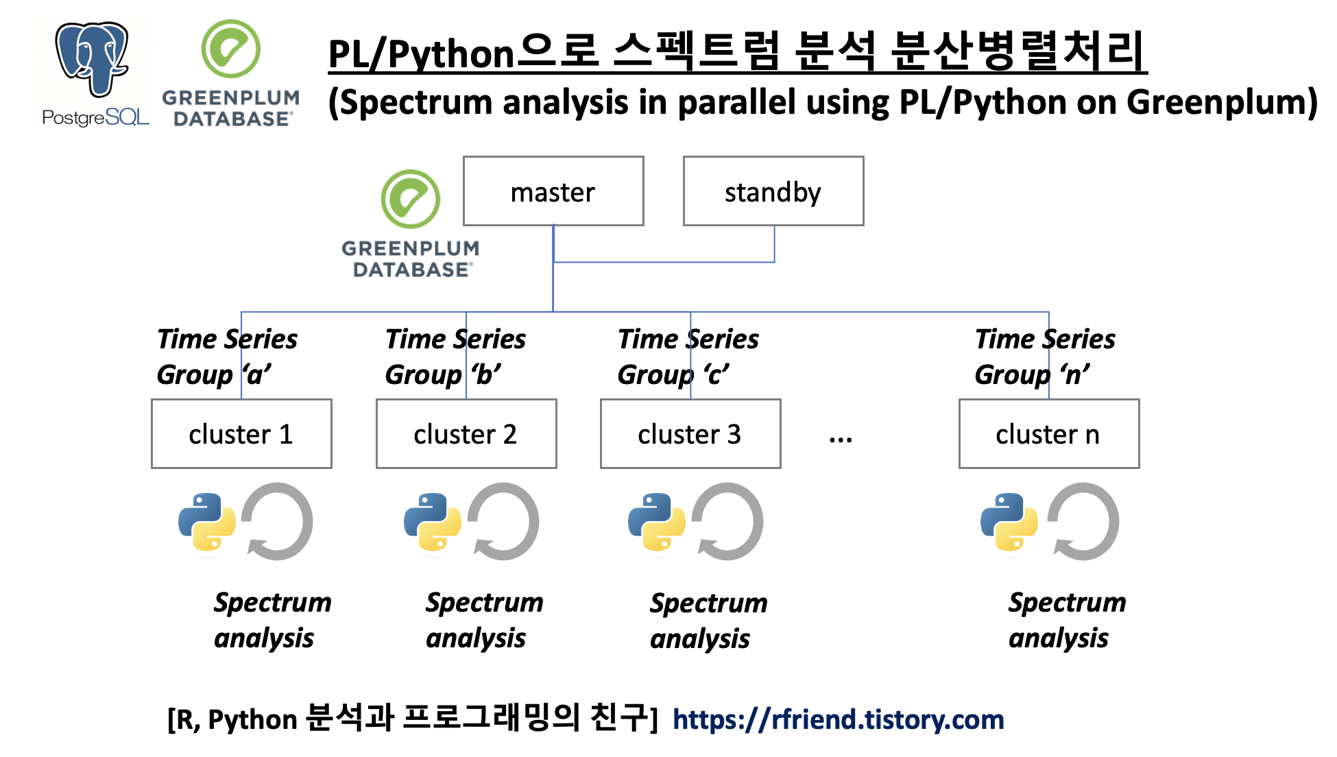
이전 포스팅에서 스펙트럼 분석(spectrum analysis, spectral analysis, frequency domain analysis) 에 대해서 소개하였습니다. ==> https://rfriend.tistory.com/690 참조
이번 포스팅에서는 Greenplum 에서 PL/Python (Procedural Language)을 활용하여 여러개 그룹의 시계열 데이터에 대해 스펙트럼 분석을 분산병렬처리하는 방법을 소개하겠습니다. (spectrum analysis in parallel using PL/Python on Greenplum database)
spectrum analysis in parallel using PL/Python on Greenplum
(1) 다른 주파수를 가진 3개 그룹의 샘플 데이터셋 생성
먼저, spectrum 모듈에서 data_cosine() 메소드를 사용하여 주파수(frequency)가 100, 200, 250 인 3개 그룹의 코사인 파동 샘플 데이터를 생성해보겠습니다. (노이즈 A=0.1 만큼이 추가된 1,024개 코사인 데이터 포인트를 가진 예제 데이터)
## generating 3 cosine signals with frequency of (100Hz, 200Hz, 250Hz) respectively
## buried in white noise (amplitude 0.1), a length of N=1024 and the sampling is 1024Hz.
from spectrum import data_cosine

data1 = data_cosine(N=1024, A=0.1, sampling=1024, freq=100)
data2 = data_cosine(N=1024, A=0.1, sampling=1024, freq=200)
data3 = data_cosine(N=1024, A=0.1, sampling=1024, freq=250)
다음으로 Python pandas 모듈을 사용해서 'grp' 라는 칼럼에 'a', 'b', 'c'의 구분자를 추가하고, 'val' 칼럼에는 위에서 생성한 각기 다른 주파수를 가지는 3개의 샘플 데이터셋을 값으로 가지는 DataFrame을 생성합니다.
## making a pandas DataFrame with a group name
import pandas as pd

df1 = pd.DataFrame({'grp': 'a', 'val': data1})
df2 = pd.DataFrame({'grp': 'b', 'val': data2})
df3 = pd.DataFrame({'grp': 'c', 'val': data3})

df = pd.concat([df1, df2, df3])


df.shape
# (3072, 2)


df.head()
# 	grp	val
# 0	a	1.056002
# 1	a	0.863020
# 2	a	0.463375
# 3	a	-0.311347
# 4	a	-0.756723
sqlalchemy 모듈의 create_engine("driver://user:password@host:port/database") 메소드를 사용해서 Greenplum 데이터베이스에 접속한 후에 pandas의 DataFrame.to_sql() 메소드를 사용해서 위에서 만든 pandas DataFrame을 Greenplum DB에 import 하도록 하겠습니다.
이때 index = True, indx_label = 'id' 를 꼭 설정해주어야만 합니다. 그렇지 않을 경우 Greenplum DB에 데이터가 import 될 때 시계열 데이터의 특성이 sequence 가 없이 순서가 뒤죽박죽이 되어서, 이후에 스펙트럼 분석을 할 수 없게 됩니다.
## importing data to Greenplum using pandas
import sqlalchemy
from sqlalchemy import create_engine

# engine = sqlalchemy.create_engine("postgresql://user:password@host:port/database")
engine = create_engine("postgresql://user:password@ip:5432/database") # set with yours

df.to_sql(name = 'data_cosine',
          con = engine,
          schema = 'public',
          if_exists = 'replace', # {'fail', 'replace', 'append'), default to 'fail'
          index = True,
          index_label = 'id',
          chunksize = 100,
          dtype = {
              'id': sqlalchemy.types.INTEGER(),
              'grp': sqlalchemy.types.TEXT(),
              'val': sqlalchemy.types.Float(precision=6)
          })


SELECT * FROM data_cosine order by grp, id LIMIT 5;
# id	grp	val
# 0	a	1.056
# 1	a	0.86302
# 2	a	0.463375
# 3	a	-0.311347
# 4	a	-0.756723


SELECT count(1) AS cnt FROM data_cosine;
# cnt
# 3072
(2) 스펙트럼 분석을 분산병렬처리하는 PL/Python 사용자 정의 함수 정의 (UDF definition)
아래의 스펙트럼 분석은 Python scipy 모듈의 signal() 메소드를 사용하였습니다. (spectrum 모듈의 Periodogram() 메소드를 사용해도 동일합니다. https://rfriend.tistory.com/690 참조)
(Greenplum database의 master node와 segment nodes 에는 numpy와 scipy 모듈이 각각 미리 설치되어 있어야 합니다.)
사용자 정의함수의 인풋으로는 (a) 시계열 데이터 array 와 (b) sampling frequency 를 받으며, 아웃풋으로는 스펙트럼 분석을 통해 추출한 주파수(frequency, spectrum)를 텍스트(혹은 int)로 반환하도록 하였습니다.
DROP FUNCTION IF EXISTS spectrum_func(float8[], int);
CREATE OR REPLACE FUNCTION spectrum_func(x float8[], fs int)
RETURNS text
AS $$
    from scipy import signal
    import numpy as np

    # x: Time series of measurement values
    # fs: Sampling frequency of the x time series. Defaults to 1.0.
    f, PSD = signal.periodogram(x, fs=fs)
    freq = np.argmax(PSD)

    return freq

$$ LANGUAGE 'plpythonu';
(3) 스펙트럼 분석을 분산병렬처리하는 PL/Python 사용자 정의함수 실행 (Execution of Spectrum Analysis in parallel on Greenplum)
위의 (2)번에서 정의한 스펙트럼 분석 PL/Python 사용자 정의함수 spectrum_func(x, fs) 를 Select 문으로 호출하여 실행합니다. FROM 절에는 sub query로 input에 해당하는 시계열 데이터를 ARRAY_AGG() 함수를 사용해 array 로 묶어주는데요, 이때 ARRAY_AGG(val::float8 ORDER BY id) 로 id 기준으로 반드시 시간의 순서에 맞게 정렬을 해주어야 제대로 스펙트럼 분석이 진행이 됩니다.
SELECT
    grp
    , spectrum_func(val_agg, 1024)::int AS freq
FROM (
    SELECT
        grp
        , ARRAY_AGG(val::float8 ORDER BY id) AS val_agg
    FROM data_cosine
    GROUP BY grp
) a
ORDER BY grp;

# grp	freq
# a	100
# b	200
# c	250
우리가 (1)번에서 주파수가 각 100, 200, 250인 샘플 데이터셋을 만들었는데요, 스펙트럼 분석을 해보니 정확하게 주파수를 도출해 내었네요!.
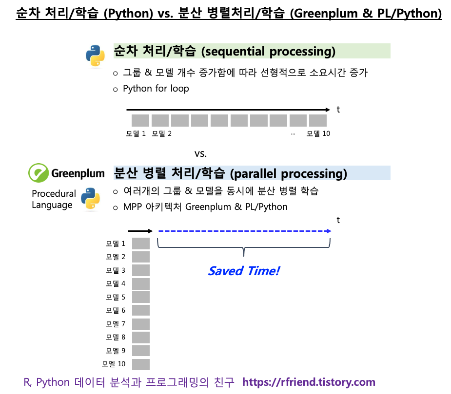
지난번 포스팅에서는 Python의 statsmodels 모듈을 이용하여 여러개의 숫자형 변수에 대해 집단 간 평균의 차이가 있는지를 for loop 순환문을 사용하여 검정하는 방법(rfriend.tistory.com/639)을 소개하였습니다.
Python에서 for loop 문을 사용하면 순차적으로 처리 (sequential processing) 를 하게 되므로, 일원분산분석을 해야 하는 숫자형 변수의 개수가 많아질 수록 선형적으로 처리 시간이 증가하게 됩니다.
Greenplum에서 PL/Python (또는 PL/R) 을 사용하면 일원분산분석의 대상의 되는 숫자형 변수가 매우 많고 데이터 크기가 크더라도 분산병렬처리 (distributed parallel processing) 하여 ANOVA test 를 처리할 수 있으므로 신속하게 분석을 할 수 있는 장점이 있습니다.
더불어서, 데이터가 저장되어 있는 DB에서 데이터의 이동 없이(no data I/O, no data movement), In-DB 처리/분석이 되므로 work-flow 가 간소화되고 batch scheduling 하기에도 편리한 장점이 있습니다.
만약 데이터는 DB에 있고, 애플리케이션도 DB를 바라보고 있고, 분석은 Python 서버 (또는 R 서버)에서 하는 경우라면, 분석을 위해 DB에서 데이터를 samfile 로 떨구고, 이를 Python에서 pd.read_csv()로 읽어들여서 분석하고, 다시 결과를 text file로 떨구고, 이 text file을 ftp로 DB 서버로 이동하고, psql로 COPY 문으로 테이블에 insert 하는 workflow ... 관리 포인트가 많아서 정신 사납고 복잡하지요?!
자, 이제 Greenplum database에서 PL/Python으로 일원분산분석을 병렬처리해서 집단 간 여러개의 개별 변수별 평균 차이가 있는지 검정을 해보겠습니다.
(1) 여러 개의 변수를 가지는 샘플 데이터 만들기
정규분포로 부터 난수를 발생시켜서 3개 그룹별로 각 30개 씩의 샘플 데이터를 생성하였습니다. 숫자형 변수로는 'x1', 'x2', 'x3', 'x4'의 네 개의 변수를 생성하였습니다. 이중에서 'x1', 'x2'는 3개 집단이 모두 동일한 평균과 분산을 가지는 정규분포로 부터 샘플을 추출하였고, 반면에 'x3', 'x4'는 3개 집단 중 2개는 동일한 평균과 분산의 정규분포로 부터 샘플을 추출하고 나머지 1개 집단은 다른 평균을 가지는 정규분포로 부터 샘플을 추출하였습니다. (뒤에 one-way ANOVA 검정을 해보면 'x3', 'x4'에 대한 집단 간 평균 차이가 있는 것으로 결과가 나오겠지요?!)
import numpy as np
import pandas as pd

# generate 90 IDs
id = np.arange(90) + 1

# Create 3 groups with 30 observations in each group.
from itertools import chain, repeat
grp = list(chain.from_iterable((repeat(number, 30) for number in [1, 2, 3])))

# generate random numbers per each groups from normal distribution
np.random.seed(1004)

# for 'x1' from group 1, 2 and 3
x1_g1 = np.random.normal(0, 1, 30)
x1_g2 = np.random.normal(0, 1, 30)
x1_g3 = np.random.normal(0, 1, 30)

# for 'x2' from group 1, 2 and 3
x2_g1 = np.random.normal(10, 1, 30)
x2_g2 = np.random.normal(10, 1, 30)
x2_g3 = np.random.normal(10, 1, 30)

# for 'x3' from group 1, 2 and 3
x3_g1 = np.random.normal(30, 1, 30)
x3_g2 = np.random.normal(30, 1, 30)
x3_g3 = np.random.normal(50, 1, 30)

# different mean
x4_g1 = np.random.normal(50, 1, 30)
x4_g2 = np.random.normal(50, 1, 30)
x4_g3 = np.random.normal(20, 1, 30)

# different mean # make a DataFrame with all together
df = pd.DataFrame({
    'id': id, 'grp': grp,
    'x1': np.concatenate([x1_g1, x1_g2, x1_g3]),
    'x2': np.concatenate([x2_g1, x2_g2, x2_g3]),
    'x3': np.concatenate([x3_g1, x3_g2, x3_g3]),
    'x4': np.concatenate([x4_g1, x4_g2, x4_g3])})


df.head()
id
grp
x1
x2
x3
x4
1
1
0.594403
10.910982
29.431739
49.232193
2
1
0.402609
9.145831
28.548873
50.434544
3
1
-0.805162
9.714561
30.505179
49.459769
4
1
0.115126
8.885289
29.218484
50.040593
5
1
-0.753065
10.230208
30.072990
49.601211
위에서 만든 가상의 샘플 데이터를 Greenplum DB에 'sample_tbl' 이라는 이름의 테이블로 생성해보겠습니다. Python pandas의 to_sql() 메소드를 사용하면 pandas DataFrame을 쉽게 Greenplum DB (또는 PostgreSQL DB)에 uploading 할 수 있습니다.
# creating a table in Greenplum by importing pandas DataFrame
conn = "postgresql://gpadmin:changeme@localhost:5432/demo"

df.to_sql('sample_tbl',
         conn,
         schema = 'public',
         if_exists = 'replace',
         index = False)
Jupyter Notebook에서 Greenplum DB에 접속해서 SQL로 이후 작업을 진행하겠습니다.
PL/Python에서 작업하기 쉽도록 테이블 구조를 wide format에서 long format 으로 변경하겠습니다. union all 로 해서 칼럼 갯수 만큼 위/아래로 append 해나가면 되는데요, DB 에서 이런 형식의 데이터를 관리하고 있다면 아마도 이미 long format 으로 관리하고 있을 가능성이 높습니다. (새로운 데이터가 수집되면 계속 insert into 하면서 행을 밑으로 계속 쌓아갈 것이므로...)
%%sql
-- reshaping a table from wide to long
drop table if exists sample_tbl_long;
create table sample_tbl_long as (
    select id, grp, 'x1' as col, x1 as val from sample_tbl
    union all
    select id, grp, 'x2' as col, x2 as val from sample_tbl
    union all
    select id, grp, 'x3' as col, x3 as val from sample_tbl
    union all
    select id, grp, 'x4' as col, x4 as val from sample_tbl
) distributed randomly;

 * postgresql://gpadmin:***@localhost:5432/demo
Done.
360 rows affected.


%sql select * from sample_tbl_long order by id, grp, col limit 8;

[Out]
 * postgresql://gpadmin:***@localhost:5432/demo
8 rows affected.
id	grp	col	val
1	1	x1	0.594403067344276
1	1	x2	10.9109819091195
1	1	x3	29.4317394311833
1	1	x4	49.2321928075563
2	1	x1	0.402608708677309
2	1	x2	9.14583073327387
2	1	x3	28.54887315985
2	1	x4	50.4345438286737
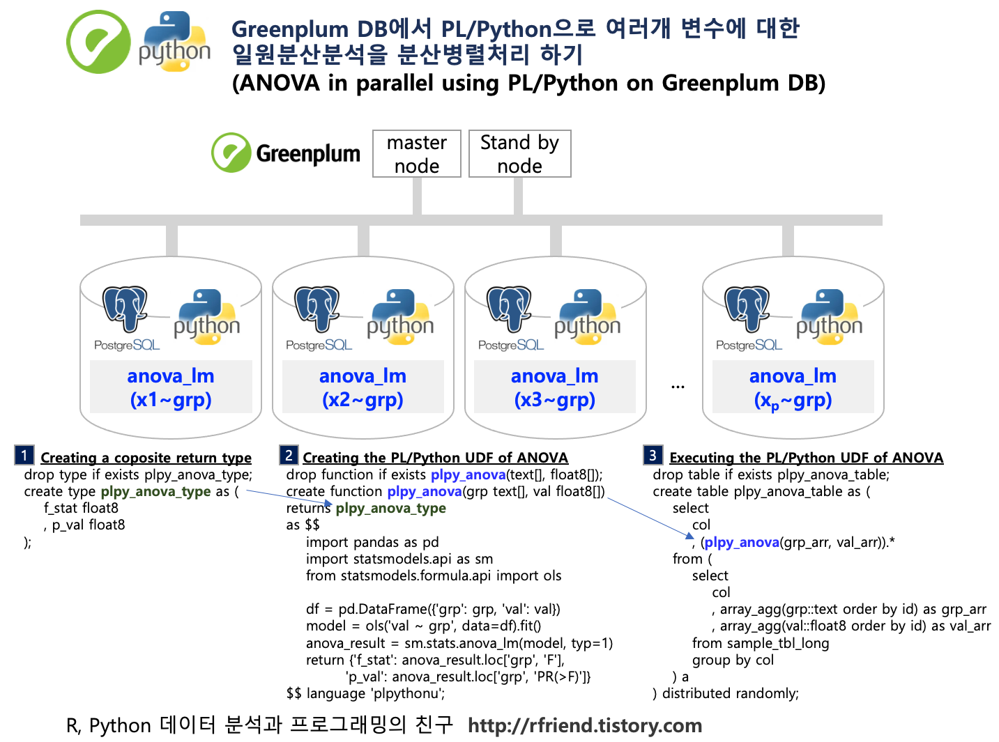
(3) 분석 결과 반환 composite type 정의
일원분산분석 결과를 반환받을 때 각 분석 대상 변수 별로 (a) F-통계량, (b) p-value 의 두 개 값을 float8 데이터 형태로 반환받는 composite type 을 미리 정의해놓겠습니다.
%%sql
-- Creating a coposite return type
drop type if exists plpy_anova_type cascade;
create type plpy_anova_type as (
    f_stat float8
    , p_val float8
);

 * postgresql://gpadmin:***@localhost:5432/demo
Done.
Done.
(4) 일원분산분석(one-way ANOVA) PL/Python 사용자 정의함수 정의
집단('grp')과 측정값('val')을 input 으로 받고, statsmodels 모듈의 sm.stats.anova_lm() 메소드로 일원분산분석을 하여 결과 테이블에서 'F-통계량'과 'p-value'만 인덱싱해서 반환하는 PL/Python 사용자 정의 함수를 정의해보겠습니다.
%%sql
-- Creating the PL/Python UDF of ANOVA
drop function if exists plpy_anova_func(text[], float8[]);
create or replace function plpy_anova_func(grp text[], val float8[])
returns plpy_anova_type
as $$
    import pandas as pd
    import statsmodels.api as sm
    from statsmodels.formula.api import ols

    df = pd.DataFrame({'grp': grp, 'val': val})
    model = ols('val ~ grp', data=df).fit()
    anova_result = sm.stats.anova_lm(model, typ=1)
    return {'f_stat': anova_result.loc['grp', 'F'],
            'p_val': anova_result.loc['grp', 'PR(>F)']}
$$ language 'plpythonu';

 * postgresql://gpadmin:***@localhost:5432/demo
Done.
Done.
(5) 일원분산분석(one-way ANOVA) PL/Python 함수 분산병렬처리 실행
PL/Python 사용자 정의함수는 SQL query 문으로 실행합니다. 이때 PL/Python 이 'F-통계량'과 'p-value'를 반환하도록 UDF를 정의했으므로 아래처럼 (plpy_anova_func(grp_arr, val_arr)).* 처럼 ().* 으로 해서 모든 결과('F-통계량' & 'p-value')를 반환하도록 해줘야 합니다. (빼먹고 실수하기 쉬우므로 ().*를 빼먹지 않도록 주의가 필요합니다)
이렇게 하면 변수별로 segment nodes 에서 분산병렬로 각각 처리가 되므로, 변수가 수백~수천개가 있더라도 (segment nodes가 많이 있다는 가정하에) 분산병렬처리되어 신속하게 분석을 할 수 있습니다. 그리고 결과는 바로 Greenplum DB table에 적재가 되므로 이후의 application이나 API service에서 가져다 쓰기에도 무척 편리합니다.
%%sql
-- Executing the PL/Python UDF of ANOVA
drop table if exists plpy_anova_table;
create table plpy_anova_table as (
    select
        col
        , (plpy_anova_func(grp_arr, val_arr)).*
    from (
        select
            col
            , array_agg(grp::text order by id) as grp_arr
            , array_agg(val::float8 order by id) as val_arr
        from sample_tbl_long
        group by col
    ) a
) distributed randomly;

 * postgresql://gpadmin:***@localhost:5432/demo
Done.
4 rows affected.
총 4개의 각 변수별 일원분산분석 결과를 조회해보면 아래와 같습니다.
%%sql
select * from plpy_anova_table order by col;

[Out]
 * postgresql://gpadmin:***@localhost:5432/demo
4 rows affected.
col	f_stat	p_val
x1	0.773700830155438	0.46445029458511966
x2	0.20615939957339052	0.8140997216173114
x3	4520.512608893724	1.2379278415456727e-88
x4	9080.286130418674	1.015467388498996e-101
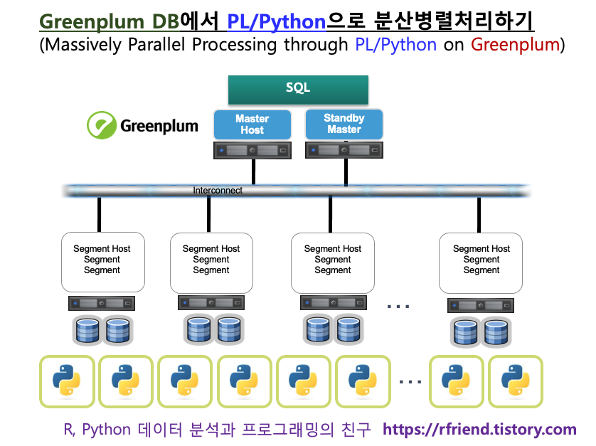
Greenplum DB는 여려개의 PostgreSQL DB를 합쳐놓은 shared-nothing architecture 의 MPP (Massively Parallel Processing) Database 입니다. 손과 발이 되는 여러개의 cluster nodes에 머리가 되는 Master host 가 조율/조정/지시해가면서 분산하여 병렬로 일을 시키고, 각 cluster nodes의 연산처리 결과를 master host 가 모아서 취합하여 최종 결과를 반환하는 방식으로 일을 하기 때문에 (1) 대용량 데이터도 (2) 매우 빠르게 처리할 수 있습니다.
이번 포스팅에서는 여기에서 한발 더 나아가서, Procedural Language Extension (PL/X) 을 사용하여 Python, R, Java, C, Perl, SQL 등의 프로그래밍 언어를 Greenplum DB 내에서 사용하여 데이터의 이동 없이 분산 병렬처리하는 방법을 소개하겠습니다.
Massively Parallel Processing through PL/Python on Greenplum DB
난수를 발생시켜서 만든 가상의 데이터셋을 사용하여 PL/Python으로 Random Forest의 Feature Importance를 숫자형 목표변수('y1_num') 그룹과 범주형 목표변수('y2_cat') 그룹 별로 분산병렬처리하는 간단한 예를 들어보겠습니다.
(b) y2_cat = case when (x4*7.0 + x5*6.0 - x6*4.0 + x4*5.0 + 0.001*random()) >= 9 then 1 else 0 의 함수로 부터 만듦.
(2) PL/Python 함수 정의하기 : (a) 숫자형 목표변수('y1_num') 그룹은 Random Forest Regressor를, (b) 범주형 목표변수('y2_cat') 그룹은 Random Forest Classifier 를 각 그룹별로 분산병렬로 훈련시킨 후, : 각 그룹별 Random Forest Regressor 모델별 200개의 숫자형 변수별 Feature Importance를 반환
(3) PL/Python 함수 실행하기
(4) 각 그룹별 변수별 Random Forest 의 Feature Importance 를 조회하기
를 해 보겠습니다.
(1) 가상의 예제 데이터셋 만들기
- group: 2개의 그룹
(목표변수로 하나는 숫자형, 하나는 범주형 값을 가지는 2개의 X&y 데이터셋 그룹을 생성함.)
(b) y2_cat = case when (x4*7.0 + x5*6.0 - x6*4.0 + x4*5.0 + 0.001*random()) >= 9 then 1 else 0
(y1_num, y2_cat 값을 만들때 x 변수에 곱하는데 사용한 *7.0, *6.0, *5.0 은 아무런 의미 없습니다.
그냥 가상의 예제 샘플 데이터를 만들려고 임의로 선택해서 곱해준 값입니다.)
아래의 예제는 In-DB 처리를 염두에 두고, 200개의 숫자형 X 변수들과 한개의 숫자형 y 변수를 DB의 테이블에 "col_nm"이라는 칼럼에는 변수 이름을, "col_val"에는 변수 값을 long form 으로 생성해서 저장해 놓은 것입니다.
나중에 PL/Python의 함수 안에서 pandas 의 pivot_table() 함수를 사용해서 wide form 으로 DataFrame의 형태를 재구조화해서 random forest 를 분석하게 됩니다.
제 맥북에서 도커로 만든 Greenplum 에는 1개의 master node와 2개의 segment nodes 가 있는데요, 편의상 cross join 으로 똑같은 칼럼과 값을 가지는 설명변수 X 데이터셋을 2의 segment nodes에 replication 해서 그룹1('grp=1'), 그룹2('grp=2')를 만들었습니다.
그리고 여기에 목표변수 y 값으로는 숫자형 목표변수 'y1_num' 칼럼의 값에 대해서는 그룹1('grp=1'), 범주형 목표변수 'y2_cat' 칼럼의 값에 대해서는 그룹2('grp=2')를 부여한 후에, 앞서 만든 설명변수 X 데이터셋에 union all 로 'y1_num'과 'y2_cat' 데이터를 합쳐서 최종으로 하나의 long format의 테이블을 만들었습니다.
첫번째 그룹은 200개의 숫자형 X 변수 중에서 'x1', 'x2', 'x3'의 3개 변수만 숫자형 목표변수(numeric target variable) 인 'y1_num'과 관련이 있고, 나머지 194개의 설명변수와는 관련이 없게끔 y1_num = x1*7.0 + x2*6.0 + x3*5.0 + 0.001*random() 함수를 사용해서 'y1_num' 을 만들었습니다 (*7.0, *6.0, *5.0 은 가상의 예제 데이터를 만들기 위해 임의로 선택한 값으로서, 아무 이유 없습니다). 뒤에서 PL/Python으로 Random Forest Regressor 의 feature importance 결과에서 'x1', 'x2', 'x3' 변수의 Feature Importance 값이 높게 나오는지 살펴보겠습니다.
두번째 그룹은 200개의 숫자형 X변수 중에서 'x4', 'x5', 'x6'의 3개 변수만 범주형 목표변수(categorical target variable) 인 'y2_cat'과 관련이 있고, 나머지 194개의 설명변수와는 연관이 없게끔 y2_cat = case when (x4*7.0 + x5*6.0 - x6*4.0 + x4*5.0 + 0.001*random()) >= 9 then 1 else 0 함수로 부터 가상으로 생성하였습니다. 뒤에서 PL/Python으로 Random Forest Classifier 의 feature importance 결과에서 'x4', 'x5', 'x6' 변수의 Feature Importance 값이 높게 나오는지 살펴보겠습니다.
------------------------------------------------------------------
-- Random Forest's Feature Importance using PL/Python on Greenplum
------------------------------------------------------------------

-- (1) Generate sample data
-- 2 groups
-- 100 observations(ID) per group
-- X: 200 numeric input variables per observation(ID)
-- y : a numeric target variable by a function of y = x1*5.0 + x2*4.5 - x3*4.0 + x4*3.5 + 0.001*random()
-- distributed by 'grp' (group)

-- (1-1) 100 IDs of observations
drop table if exists id_tmp;
create table id_tmp (
	id integer
) distributed randomly;

insert into id_tmp (select * from generate_series(1, 100, 1));

select * from id_tmp order by id limit 3;
--id
--1
--2
--3


-- (1-2) 200 X variables
drop table if exists x_tmp;
create table x_tmp (
	x integer
) distributed randomly;

insert into x_tmp (select * from generate_series(1, 200, 1));

select * from x_tmp order by x limit 3;
--x
--1
--2
--3


-- (1-3) Cross join of ID and Xs
drop table if exists id_x_tmp;
create table id_x_tmp as (
	select * from id_tmp
	cross join x_tmp
) distributed randomly;

select count(1) from id_x_tmp;
-- 20,000  -- (id 100 * x 200 = 20,000)

select * from id_x_tmp order by id, x limit 3;
--id  x
--1	  1
--1	  2
--1	  3


-- (1-4) Generate X values randomly
drop table if exists x_long_tmp;
create table x_long_tmp as (
	select
		a.id as id
		, x
		, 'x'||a.x::text as x_col
		, round(random()::numeric, 3) as x_val
	from id_x_tmp a
) distributed randomly;

select count(1) from x_long_tmp;
-- 20,000

select * from x_long_tmp order by id, x limit 3;
--id  x  x_col  x_val
--1	  1	 x1	    0.956
--1	  2	 x2	    0.123
--1	  3	 x3	    0.716

select min(x_val) as x_min_val, max(x_val) as x_max_val from x_long_tmp;
--x_min_val  x_max_val
--0.000	     1.000


-- (1-5) create y values
drop table if exists y_tmp;
create table y_tmp as (
	select
		s.id
		, (s.x1*7.0 + s.x2*6.0 + s.x3*5.0 + 0.001*random()) as y1_num -- numeric
		, case when (s.x4*7.0 + s.x5*6.0 + s.x6*5.0 + 0.001*random()) >= 9
			then 1
			else 0
			end as y2_cat -- categorical
	from (
		select distinct(a.id) as id, x1, x2, x3, x4, x5, x6 from x_long_tmp as a
		left join (select id, x_val as x1 from x_long_tmp where x_col = 'x1') b
			on a.id = b.id
		left join (select id, x_val as x2 from x_long_tmp where x_col = 'x2') c
			on a.id = c.id
		left join (select id, x_val as x3 from x_long_tmp where x_col = 'x3') d
			on a.id = d.id
		left join (select id, x_val as x4 from x_long_tmp where x_col = 'x4') e
			on a.id = e.id
		left join (select id, x_val as x5 from x_long_tmp where x_col = 'x5') f
			on a.id = f.id
		left join (select id, x_val as x6 from x_long_tmp where x_col = 'x6') g
			on a.id = g.id
	) s
) distributed randomly;

select count(1) from y_tmp;
--100

select * from y_tmp order by id limit 5;
--id  y1_num            y2_cat
--1	11.0104868695838	1
--2	10.2772997177048	0
--3	7.81790575686749	0
--4	8.89387259676540	1
--5	2.47530914815422	1


--  (1-6) replicate X table to all clusters
--        by the number of 'y' varialbes. (in this case, there are 2 y variables, 'y1_num' and 'y2_cat'
drop table if exists long_x_grp_tmp;
create table long_x_grp_tmp as (
	select
		b.grp as grp
		, a.id as id
		, a.x_col as col_nm
		, a.x_val as col_val
	from x_long_tmp as a
	cross join (
		select generate_series(1, c.y_col_cnt) as grp
		from (
			select (count(distinct column_name) - 1) as y_col_cnt
			from information_schema.columns
				where table_name = 'y_tmp' and table_schema = 'public') c
		) as b -- number of clusters
) distributed randomly;


select count(1) from long_x_grp_tmp;
-- 40,000   -- 2 (y_col_cnt) * 20,000 (x_col_cnt)

select * from long_x_grp_tmp order by id limit 5;
--grp  id   col_nm  col_val
--1	1	x161	0.499
--2	1	x114	0.087
--1	1	x170	0.683
--2	1	x4	    0.037
--2	1	x45	    0.995


-- (1-7) create table in long format with x and y
drop table if exists long_x_y;
create table long_x_y as (
	select x.*
	from long_x_grp_tmp as x
	union all
	select 1::int as grp, y1.id as id, 'y1_num'::text as col_nm, y1.y1_num as col_val
	from y_tmp as y1
	union all
	select 2::int as grp, y2.id as id, 'y2_cat'::text as col_nm, y2.y2_cat as col_val
	from y_tmp as y2
) distributed randomly;

select count(1) from long_x_y;
-- 40,200 (x 40,000 + y1_num 100 + y2_cat 100)

select grp, count(1) from long_x_y group by 1 order by 1;
--grp  count
--1	   20100
--2	   20100

select * from long_x_y where grp=1 order by id, col_nm desc limit 5;
--grp  id   col_nm  col_val
--1	   1	y1_num	11.010
--1	   1	x99	     0.737
--1	   1	x98	     0.071
--1	   1	x97	     0.223
--1	   1	x96	     0.289

select * from long_x_y where grp=2 order by id, col_nm desc limit 5;
--grp  id   col_nm  col_val
--2	   1	y2_cat	1.0
--2	   1	x99	    0.737
--2	   1	x98	    0.071
--2	   1	x97	    0.223
--2	   1	x96	    0.289


-- drop temparary tables
drop table if exists id_tmp;
drop table if exists x_tmp;
drop table if exists id_x_tmp;
drop table if exists x_long_tmp;
drop table if exists y_tmp;
drop table if exists long_x_grp_tmp;
(2) PL/Python 사용자 정의함수 정의하기
- (2-1) composite return type 정의하기
PL/Python로 분산병렬로 연산한 Random Forest의 feature importance (또는 variable importance) 결과를 반환할 때 텍스트 데이터 유형의 '목표변수 이름(y_col_nm)', '설명변수 이름(x_col_nm)'과 '변수 중요도(feat_impo)' 의 array 형태로 반환하게 됩니다. 반환하는 데이터가 '텍스트'와 'float8' 로 서로 다른 데이터 유형이 섞여 있으므로 composite type 의 return type 을 만들어줍니다. 그리고 PL/Python은 array 형태로 반환하므로 text[], text[] 과 같이 '[]' 로서 array 형태로 반환함을 명시합니다.
-- define composite return type
drop type if exists plpy_rf_feat_impo_type cascade;
create type plpy_rf_feat_impo_type as (
	y_col_nm text[]
	, x_col_nm text[]
	, feat_impo float8[]
);
- (2-2) Random Forest feature importance 결과를 반환하는 PL/Python 함수 정의하기
PL/Python 사용자 정의 함수를 정의할 때는 아래와 같이 PostgreSQL의 Procedural Language 함수 정의하는 표준 SQL 문을 사용합니다.
input data 는 array 형태이므로 칼럼 이름 뒤에 데이터 유형에는 '[]'를 붙여줍니다.
중간의 $$ ... python code block ... $$ 부분에 pure python code 를 넣어줍니다.
제일 마지막에 PL/X 언어로서 language 'plpythonu' 으로 PL/Python 임을 명시적으로 지정해줍니다.
create or replace function function_name(column1 data_type1[], column2 data_type2[], ...) returns return_type as $$ ... python code block ... $$ language 'plpythonu';
만약 PL/Container 를 사용한다면 명령 프롬프트 창에서 아래처럼 $ plcontainer runtime-show 로 Runtime ID를 확인 한 후에,
PL/Python 코드블록의 시작 부분에 $$ # container: container_Runtime_ID 로서 사용하고자 하는 docker container 의 runtime ID를 지정해주고, 제일 마지막 부분에 $$ language 'plcontainer'; 로 확장 언어를 'plcontainer'로 지정해주면 됩니다. PL/Container를 사용하면 최신의 Python 3.x 버전을 사용할 수 있는 장점이 있습니다.
create or replace function function_name(column1 data_type1[], column2 data_type2[], ...) returns return_type as $$ # container: plc_python3_shared ... python code block ... $$ LANGUAGE 'plcontainer';
아래 코드에서는 array 형태의 'id', 'col_nm', 'col_val'의 3개 칼럼을 input 으로 받아서 먼저 pandas DataFrame으로 만들어 준 후에, 이를 pandas pivot_table() 함수를 사용해서 long form --> wide form 으로 데이터를 재구조화 해주었습니다.
다음으로, 숫자형의 목표변수('y1_num')를 가지는 그룹1 데이터셋에 대해서는 sklearn 패키지의 RandomForestRegressor 클래스를 사용해서 Random Forest 모델을 훈련하고, 범주형의 목표변수('y2_cat')를 가지는 그룹2의 데이터셋에 대해서는 sklearn 패키지의 RandomForestClassifier 클래스를 사용하여 모델을 훈련하였습니다. 그리고 'rf_regr_fitted.feature_importances_' , 'rf_clas_fitted.feature_importances_'를 사용해서 200개의 각 변수별 feature importance 속성을 리스트로 가져왔습니다.
마지막에 return {'y_col_nm': y_col_nm, 'x_col_nm': x_col_nm_list, 'feat_impo': feat_impo} 에서 전체 변수 리스트와 변수 중요도 연산 결과를 array 형태로 반환하게 했습니다.
----------------------------------
-- PL/Python UDF for Random Forest
----------------------------------

-- define PL/Python function
drop function if exists plpy_rf_feat_impo_func(text[], text[], text[]);
create or replace function plpy_rf_feat_impo_func(
	id_arr text[]
	, col_nm_arr text[]
	, col_val_arr text[]
) returns plpy_rf_feat_impo_type as
$$
#import numpy as np
import pandas as pd

# making a DataFrame
xy_df = pd.DataFrame({
    'id': id_arr
    , 'col_nm': col_nm_arr
    , 'col_val': col_val_arr
})

# pivoting a table
xy_pvt = pd.pivot_table(xy_df
                        , index = ['id']
                        , columns = 'col_nm'
                        , values = 'col_val'
                        , aggfunc = 'first'
                        , fill_value = 0)

X = xy_pvt[xy_pvt.columns.difference(['y1_num', 'y2_cat'])]
X = X.astype(float)
x_col_nm_list = X.columns

# UDF for Feature Importance by RandomForestRegressor
def rf_regr_feat_impo(X, y):

	# training RandomForestRegressor
	from sklearn.ensemble import RandomForestRegressor
	rf_regr = RandomForestRegressor(n_estimators=200)
	rf_regr_fitted = rf_regr.fit(X, y)

	# The impurity-based feature importances.
	rf_regr_feat_impo = rf_regr_fitted.feature_importances_
	return rf_regr_feat_impo


# UDF for Feature Importance by RandomForestClassifier
def rf_clas_feat_impo(X, y):

	# training  RandomForestClassifier with balanced class_weight
	from sklearn.ensemble import RandomForestClassifier
	rf_clas = RandomForestClassifier(n_estimators=200, class_weight='balanced')
	rf_clas_fitted = rf_clas.fit(X, y)

	# The impurity-based feature importances.
	rf_clas_feat_impo = rf_clas_fitted.feature_importances_
	return rf_clas_feat_impo


# training RandomForest and getting variable(feature) importance
if 'y1_num' in xy_pvt.columns:
	y_target = 'y1_num'
	y = xy_pvt[y_target]
	feat_impo = rf_regr_feat_impo(X, y)

if 'y2_cat' in xy_pvt.columns:
	y_target = 'y2_cat'
	y = xy_pvt[y_target]
	y = y.astype(int)
	feat_impo = rf_clas_feat_impo(X, y)

feat_impo_df = pd.DataFrame({
	'y_col_nm': y_target
	, 'x_col_nm': x_col_nm_list
	, 'feat_impo': feat_impo
})

# returning the results of feature importances
return {
	'y_col_nm': feat_impo_df['y_col_nm']
	, 'x_col_nm': feat_impo_df['x_col_nm']
	, 'feat_impo': feat_impo_df['feat_impo']
	}

$$ language 'plpythonu';
(3) PL/Python 함수 실행하기
PL/Python 함수를 실행할 때는 표준 SQL Query 문의 "SELECT group_name, pl_python_function() FROM table_name" 처럼 함수를 SELECT 문으로 직접 호출해서 사용합니다.
PL/Python의 input 으로 array 형태의 데이터를 넣어주므로, 아래처럼 FROM 절의 sub query 에 array_agg() 함수로 먼저 데이터를 'grp' 그룹 별로 array aggregation 하였습니다.
PL/Python 함수의 전체 결과를 모두 반환할 것이므로(plpy_rf_var_impo_func()).* 처럼 함수를 모두 감싼 후에 ().* 를 사용하였습니다. (실수해서 빼먹기 쉬우므로 유의하시기 바랍니다.)
목표변수가 숫자형('y1_num')과 범주형('y2_cat')'별로 그룹1과 그룹2로 나누어서, 'grp' 그룹별로 분산병렬로 Random Forest 분석이 진행되며, Variable importance 결과를 'grp' 그룹 ID를 기준으로 분산해서 저장(distributed by (grp);)하게끔 해주었습니다.
-- execute PL/Python function
drop table if exists rf_feat_impo_result;
create table rf_feat_impo_result as (
	select
		a.grp
		, (plpy_rf_feat_impo_func(
			a.id_arr
			, a.col_nm_arr
			, a.col_val_arr
		)).*
		from (
			select
				c.grp
				, array_agg(c.id::text order by id) as id_arr
				, array_agg(c.col_nm::text order by id) as col_nm_arr
				, array_agg(c.col_val::text order by id) as col_val_arr
			from long_x_y as c
			group by grp
			) a
) distributed by (grp);
(4) 각 그룹별 변수별 Random Forest 의 Feature Importance 조회하기
위의 (3)번을 실행해서 나온 결과를 조회하면 아래와 같이 'grp=1', 'grp=2' 별로 각 칼럼별로 Random Forest에 의해 계산된 변수 중요도(variable importance) 가 array 형태로 저장되어 있음을 알 수 있습니다.
select count(1) from rf_feat_impo_result;
-- 2

-- results in array-format
select * from rf_feat_impo_result order by grp;
plpython_random_forest_feature_importance_array
위의 array 형태의 결과는 사람이 눈으로 보기에 불편하므로, unnest() 함수를 써서 long form 으로 길게 풀어서 결과를 조회해 보겠습니다.
이번 예제에서는 난수로 생성한 X설명변수에 임의로 함수를 사용해서 숫자형 목표변수('y1_num')를 가지는 그룹1에 대해서는 'x1', 'x2', 'x3' 의 순서대로 변수가 중요하고, 범주형 목표변수('y2_cat')를 가지는 그룹2에서는 'x4', 'x5', 'x6'의 순서대로 변수가 중요하게 가상의 예제 데이터셋을 만들어주었습니다. (random() 함수로 난수를 생성해서 예제 데이터셋을 만들었으므로, 매번 실행할 때마다 숫자는 달라집니다).
아래 feature importance 결과를 보니, 역시 그룹1의 데이터셋에 대해서는 'x1', 'x2', 'x3' 변수가 중요하게 나왔고, 그룹2의 데이터셋에 대해서는 'x4', 'x5', 'x6' 변수가 중요하다고 나왔네요.
-- display the results using unnest()
select
	grp
	, unnest(y_col_nm) as y_col_nm
	, unnest(x_col_nm) as x_col_nm
	, unnest(feat_impo) as feat_impo
from rf_feat_impo_result
where grp = 1
order by feat_impo desc
limit 10;
--grp    y_col_nm      x_col_nm      feat_impo
--1	   y1_num	 x1	       0.4538784064497847
--1	   y1_num	 x2	       0.1328532144509229
--1	   y1_num	 x3	       0.10484121806286809
--1	   y1_num	 x34           0.006843343319633915
--1	   y1_num	 x42           0.006804819286213849
--1	   y1_num	 x182          0.005771113354638556
--1	   y1_num	 x143          0.005220090515711377
--1	   y1_num	 x154          0.005101366229848041
--1	   y1_num	 x46           0.004571420249598611
--1	   y1_num	 x57           0.004375780774099066

select
	grp
	, unnest(y_col_nm) as y_col_nm
	, unnest(x_col_nm) as x_col_nm
	, unnest(feat_impo) as feat_impo
from rf_feat_impo_result
where grp = 2
order by feat_impo desc
limit 10;
--grp    y_col_nm      x_col_nm      feat_impo
--2	   y2_cat	 x4	       0.07490484681851341
--2	   y2_cat	 x5	       0.04099924609654107
--2	   y2_cat	 x6	       0.03431643243509608
--2	   y2_cat	 x12           0.01474464870781392
--2	   y2_cat	 x40           0.013865405628514437
--2	   y2_cat	 x37           0.013435535581862938
--2	   y2_cat	 x167          0.013236591006394367
--2	   y2_cat	 x133  	       0.012570295279560963
--2	   y2_cat	 x142  	       0.012177597741973058
--2	   y2_cat	 x116          0.011713289042962961


-- The end.