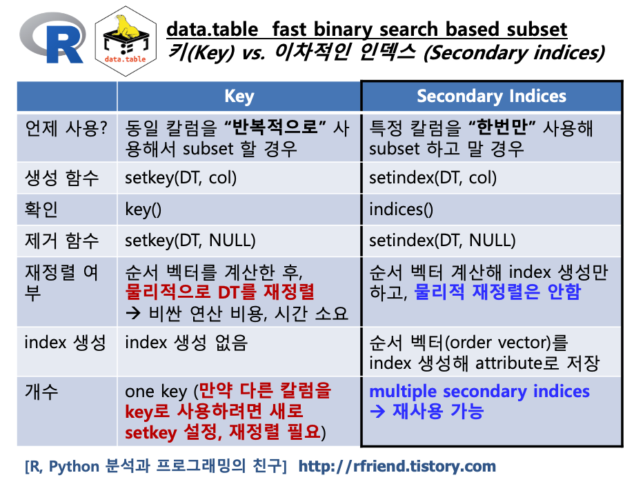
지난번 포스팅에서는 R data.table에서 (a) 키(Key)와 빠른 이진 탐색 기반의 Subsetting 하는 방법 (rfriend.tistory.com/569), (b) 2차 인덱스 (secondary indices) 를 활용하여 data.table 의 재정렬 없이 빠른 탐색 기반 Subsetting 하는 방법을 소개하였습니다. (rfriend.tistory.com/615)

이번 포스팅에서는 R data.table에서 이진 연산자(binary operators) 인 '=='와 '%in%' 를 수행하는 과정에서 이차 인덱스(secondary indices)가 자동으로 인덱싱(Auto indexing)이 되어 빠르게 subsetting 하는 내용을 소개하겠습니다. (이 글을 쓰는 2021년 2월 현재는 '=='와 '%in%' 연산자만 자동 인덱싱이 지원되며, 향후 더 많은 연산자로 확대 전망)


(1) '==' 이진 연산자로 자동 인덱싱하고 속도 비교하기

(2) '%in%' 이진 연산자로 자동 인덱싱하고 속도 비교하기

(3) 전역으로 자동 인덱싱을 비활성화하기 (disable auto indexing globally)


자동 인덱싱의 속도 개선 효과를 확인해 보기 위해서 천만개의 행을 가진 예제 data.table을 난수를 발생시켜서 생성해 보겠습니다.  DT data.table의 크기를 object.size()로 재어보니 114.4 Mb 이네요.


## =========================
## R data.table
## : Auto indexing
## =========================

library(data.table)

## create a data.table big enough
set.seed(1L)
DT = data.table(x = sample(x = 1e5L, 
                           size = 1e7L, 
                           replace = TRUE), 
                y = runif(100L))

head(DT)
#    x         y
# 1: 24388 0.4023457
# 2: 59521 0.9142361
# 3: 43307 0.2847435
# 4: 69586 0.3440578
# 5: 11571 0.1822614
# 6: 25173 0.8130521

dim(DT)
# [1] 10000000        2

print(object.size(DT), units = "Mb")
# 114.4 Mb


(1) '==' 이진 연산자로 자동 인덱싱하고 속도 비교하기


이전 포스팅의 이차 인덱스(secondary index)에서는 setindex(DT, column) 으로 이차 인덱스를 명시적으로 설정하거나, 또는 'on' 매개변수로 subsetting을 하면 실행 중에 (on the fly) 기존 이차 인덱스가 있는지 여부를 확인해서, 없으면 바로 이차 인덱스를 설정해주다고 하였습니다.

R data.table에서 '==' 이진 연산자를 사용해서 행의 부분집합을 가져오기(subsetting)을 하면 기존 이차 인덱스가 없을 경우 자동으로 인덱싱을 해줍니다. 그래서 처음에 '=='로 subsetting 할 때는 (a) 인덱스를 생성하고 + (b) 부분집합 행 가져오기 (subsetting)를 수행하느라 시간이 오래 소요되지만, 두번째로 실행할 때는 인덱스가 생성이 되어 있으므로 속도가 무척 빨라지게 됩니다!


아래의 예에서 보면 처음으로 DT[x == 500L] 을 실행했을 때는 0.406초가 소요(elapsed time)되었습니다. names(attributes(DT)) 로 확인해 보면 애초에 없던 index 가 새로 생성되었음을 확인할 수 있고, indices(DT) 로 확인해보면 "x" 칼럼에 대해 이차 인덱스가 생성되었네요.


## -- when we use '==' or '%in%' on a single column for the first time, 
## a secondary index is created automatically, and used to perform the subset. 

## have a look at all the attribute names (no index here)
names(attributes(DT))
# [1] "names"             "row.names"         "class"             ".internal.selfref"

## run the first time
## system.time = the time to create the index + the time to subset
(t1 <- system.time(ans <- DT[x == 500L]))
#  user  system elapsed 
# 0.392   0.014   0.406

head(ans)
#    x         y
# 1: 500 0.7845248
# 2: 500 0.9612705
# 3: 500 0.4023457
# 4: 500 0.9139429
# 5: 500 0.8280599
# 6: 500 0.2847435


## secondary index is created
names(attributes(DT))
# [1] "names"             "row.names"         "class"             ".internal.selfref" 
# [5] "index"

indices(DT)
# [1] "x"


이제 위에서 수행했던 연산과 동일하게 DT[x == 500L] 을 수행해서 소요 시간(elapsed time)을 측정해보면, 연속해서 두번째 수행했을 때는 0.001 초가 걸렸습니다.

## secondary indices are extremely fast in successive subsets. 
## successive subsets
(t2 <- system.time(DT[x == 500L]))
#  user  system elapsed 
# 0.001   0.000   0.001


처음 수행했을 때는 0.406초가 걸렸던 것이, 처음 수행할 때 자동 인덱싱(auto indexing)이 된 후에 연속해서 수행했을 때 0.001초가 걸려서 400배 이상 빨라졌습니다!  와우!!!


barplot(c(0.406, 0.001), 
        horiz = TRUE, 
        xlab = "elapsed time",
        col = c("red", "blue"),
        legend.text = c("first time", "second time(auto indexing)"), 
        main = "R data.table Auto Indexing")


(2) '%in%' 이진 연산자로 자동 인덱싱하고 속도 비교하기


'==' 연산자와 더불어 포함되어 있는지 여부를 확인해서 블리언을 반환하는 '%in%' 연산자를 활용해서 부분집합 행을 가져올 때도 R data.table은 자동 인덱싱(auto indexing)을 하여 이차 인덱스를 생성하고, 기존에 인덱스가 생성되어 있으면 이차 인덱스를 활용하여 빠르게 탐색하고 subsetting 결과를 반환합니다.

아래 예는 x 에 1989~2912 까지의 정수가 포함되어 있는 행을 부분집합으로 가져오기(DT[ x %in% 1989:2912]) 하는 것으로서, 이때 자동으로 인덱스를 생성(auto indexing)해 줍니다.


## '%in%' operator create auto indexing as well
system.time(DT[x %in% 1989:2912])
#  user  system elapsed 
# 0.010   0.016   0.027


행을 subsetting 할 때 사용하는 조건절이 여러개의 칼럼을 대상으로 하는 경우 '&' 연산자를 사용하여 자동 인덱싱을 할 수 있습니다.


## auto indexing to expressions involving more than one column with '&' operator
(t3 <- system.time(DT[x == 500L & y >= 0.5]))
#  user  system elapsed 
# 0.070   0.025   0.097


(3) 전역으로 자동 인덱싱을 비활성화하기 (disable auto indexing globally)


지난번 포스팅에서 지역적으로 특정 칼럼의 이차 인덱스를 제거할 때 setindex(DT, NULL) 을 사용한다고 소개하였습니다. 

(a) '전역적으로 자동 인덱싱을 비활성화' 하려면 options(datatable.auto.index = FALSE) 를 설정해주면 됩니다.

(b) '전역으로 전체 인덱스를 비활성화' 하려면 options(datatable.use.index = FALSE) 를 설정해주면 됩니다.


## Auto indexing can be disabled by setting the global argument 
options(datatable.auto.index = FALSE)

## You can disable indices fully by setting global argument
options(datatable.use.index = FALSE)


 [ Reference ]

* R data.table vignettes 'Secondary indices and auto indexing'
cran.r-project.org/web/packages/data.table/vignettes/datatable-secondary-indices-and-auto-indexing.html


이번 포스팅이 많은 도움이 되었기를 바랍니다.

행복한 데이터 과학자 되세요.  :-)


728x90
반응형
Posted by Rfriend
,

이전 포스팅에서는 R data.table에서 '키와 빠른 이진 탐색 기반의 부분집합 선택 (Key and fast binary search based subset)' 에 대해서 소개하였습니다. (rfriend.tistory.com/569)

이번 포스팅에서는 R data.table에서 '2차 인덱스 (Secondary indices)'를 사용하여 빠른 이진 탐색 기반의 부분집합 가져오기 방법을 소개하겠습니다.  이번 포스팅은 R data.table vignettes 을 참조하였습니다.


(1) 이차 인덱스 (Secondary indices) 는 무엇이, 키(Key)와는 무엇이 다른가?

(2) 이차 인덱스를 설정하고 확인하는 방법

(3) 'on' 매개변수와 이차 인덱스를 사용해서 빠르게 부분집합 가져오기

(4) Chaining 해서 정렬하기

(5) j 에 대해 계산하기 (compute or do in j)

(6) J 에 := 를 사용해서 참조하여 부분할당하기 (sub-assign by reference using := in j)

(7) by 를 사용해서 집계하기 (Aggregation using by)

(8) mult 매개변수를 사용해 첫번째 행, 마지막행 가져오기

(9) 이차 인덱스 제거하기 (remove all secondary indices)


(1) 이차 인덱스는 무엇이고, 키와는 무엇이 다른가?
    (Key vs. Secondary indices)

이차 인덱스(Secondary indices) 는 data.table의 키(Key)와 비슷하게 빠른 이진 탐색 기반의 부분집합 가져오기를 할 때 사용합니다.

하지만 키(Key)가 (a) 순서 벡터를 계산한 다음에, (b) 물리적으로 data.table을 재정렬(physically reordering)하는데 비해, 이차 인덱스(secondary indices)는 순서 벡터를 계산해서 index 를 생성해 속성으로 저장만 하고, 물리적 재정렬은 하지 않는 차이점이 있습니다. 만약 data.table의 행과 열이 매우 많은 큰 크기의 데이터셋이라면 물리적으로 재정렬하는데 많은 처리 비용과 시간이 소요될 것입니다.

또 하나 큰 차이점은, 키(Key)는 하나의 칼럼을 키로 설정했을 때 다른 칼럼을 키로 사용하려면 키를 새로운 칼럼으로 재설정하고 data.table을 물리적으로 재정렬을 해야 하는 반면에, 이차 인덱스(secondary indices)는 복수의 이차 인덱스를 설정하고 재사용할 수 있습니다.


이러한 차이점을 고려했을 때, 키(Key)는 동일 칼럼을 "반복적으로" 사용해서 빠르게 부분집합 가져오기(subsetting)를 해야 할 때 유리하며, 이차 인덱스(Secondary indices)는 복수개의 칼럼을 단발성으로 사용하면서 빠르게 부분집합 가져오기를 해야 하는 경우에 유리합니다.


[ R data.table 키(Key) vs. 이차적인 인덱스 (Secondary indices) ]


(2) 이차 인덱스를 설정하고 확인하는 방법


R data.table 패키지를 importing 하고, 예제로 사용할 데이터로는 Lahman 패키지에 들어있는 투수의 투구 통계 데이터인 "Pitching"을 참조하여 Data.Table로 불러오겠습니다.


library(data.table)

## Lahman database on baseball
#install.packages("Lahman")
library(Lahman)
data("Pitching")

## coerce lists and data.frame to data.table by reference
setDT(Pitching)

str(Pitching)
# Classes 'data.table' and 'data.frame':	47628 obs. of  30 variables:
#   $ playerID: chr  "bechtge01" "brainas01" "fergubo01" "fishech01" ...
# $ yearID  : int  1871 1871 1871 1871 1871 1871 1871 1871 1871 1871 ...
# $ stint   : int  1 1 1 1 1 1 1 1 1 1 ...
# $ teamID  : Factor w/ 149 levels "ALT","ANA","ARI",..: 97 142 90 111 90 136 111 56 97 136 ...
# $ lgID    : Factor w/ 7 levels "AA","AL","FL",..: 4 4 4 4 4 4 4 4 4 4 ...
# $ W       : int  1 12 0 4 0 0 0 6 18 12 ...
# $ L       : int  2 15 0 16 1 0 1 11 5 15 ...
# $ G       : int  3 30 1 24 1 1 3 19 25 29 ...
# $ GS      : int  3 30 0 24 1 0 1 19 25 29 ...
# $ CG      : int  2 30 0 22 1 0 1 19 25 28 ...
# $ SHO     : int  0 0 0 1 0 0 0 1 0 0 ...
# $ SV      : int  0 0 0 0 0 0 0 0 0 0 ...
# $ IPouts  : int  78 792 3 639 27 3 39 507 666 747 ...
# $ H       : int  43 361 8 295 20 1 20 261 285 430 ...
# $ ER      : int  23 132 3 103 10 0 5 97 113 153 ...
# $ HR      : int  0 4 0 3 0 0 0 5 3 4 ...
# $ BB      : int  11 37 0 31 3 0 3 21 40 75 ...
# $ SO      : int  1 13 0 15 0 0 1 17 15 12 ...
# $ BAOpp   : num  NA NA NA NA NA NA NA NA NA NA ...
# $ ERA     : num  7.96 4.5 27 4.35 10 0 3.46 5.17 4.58 5.53 ...
# $ IBB     : int  NA NA NA NA NA NA NA NA NA NA ...
# $ WP      : int  7 7 2 20 0 0 1 15 3 44 ...
# $ HBP     : int  NA NA NA NA NA NA NA NA NA NA ...
# $ BK      : int  0 0 0 0 0 0 0 2 0 0 ...
# $ BFP     : int  146 1291 14 1080 57 3 70 876 1059 1334 ...
# $ GF      : int  0 0 0 1 0 1 1 0 0 0 ...
# $ R       : int  42 292 9 257 21 0 30 243 223 362 ...
# $ SH      : int  NA NA NA NA NA NA NA NA NA NA ...
# $ SF      : int  NA NA NA NA NA NA NA NA NA NA ...
# $ GIDP    : int  NA NA NA NA NA NA NA NA NA NA ...
# - attr(*, ".internal.selfref")=<externalptr>


이차 인덱스는 setindex(DT, column) 함수의 구문으로 설정할 수 있습니다. 그러면 순서 벡터를 계산해서 내부에 index 라는 속성(attribute)을 생성해서 저장하며, 물리적으로 data.table을 재정렬하는 것은 하지 않습니다(no physical reordering)

names(attributes(DT)) 으로 확인해보면 제일 마지막에 "index"라는 속성이 추가된 것을 알 수 있습니다.  indices(DT) 함수를 사용하면 모든 이차 인덱스의 리스트를 얻을 수 있습니다.  이때 만약 아무런 이차 인덱스가 설정되어 있지 않다면 NULL 을 반환합니다.


## (1) Secondary indices
## set the column teamID as a secondary index in teh data.table Pitching
setindex(Pitching, teamID)
head(Pitching)
#    playerID yearID stint teamID lgID  W  L  G GS CG SHO SV IPouts   H  ER HR BB SO BAOpp   ERA IBB WP HBP BK  BFP GF   R SH SF
# 1: bechtge01   1871     1    PH1   NA  1  2  3  3  2   0  0     78  43  23  0 11  1    NA  7.96  NA  7  NA  0  146  0  42 NA NA
# 2: brainas01   1871     1    WS3   NA 12 15 30 30 30   0  0    792 361 132  4 37 13    NA  4.50  NA  7  NA  0 1291  0 292 NA NA
# 3: fergubo01   1871     1    NY2   NA  0  0  1  0  0   0  0      3   8   3  0  0  0    NA 27.00  NA  2  NA  0   14  0   9 NA NA
# 4: fishech01   1871     1    RC1   NA  4 16 24 24 22   1  0    639 295 103  3 31 15    NA  4.35  NA 20  NA  0 1080  1 257 NA NA
# 5: fleetfr01   1871     1    NY2   NA  0  1  1  1  1   0  0     27  20  10  0  3  0    NA 10.00  NA  0  NA  0   57  0  21 NA NA
# 6: flowedi01   1871     1    TRO   NA  0  0  1  0  0   0  0      3   1   0  0  0  0    NA  0.00  NA  0  NA  0    3  1   0 NA NA
#      GIDP
# 1:   NA
# 2:   NA
# 3:   NA
# 4:   NA
# 5:   NA
# 6:   NA


## alternatively we can provide character vectors to the function 'setindexv()'
# setindexv(Pitching, "teamID") # useful to program with

## 'index' attribute added
names(attributes(Pitching))
# [1] "names"             "row.names"         "class"             ".internal.selfref" 
# [5] "index"


## get all the secondary indices set
indices(Pitching)
# [1] "teamID"


(3) 'on' 매개변수와 이차 인덱스를 사용해서 빠르게 부분집합 가져오기


'on' 매개변수를 사용하면 별도로 setindex()로 매번 이차 인덱스를 설정하는 절차 없이, 바로 실행 중에(on the fly) 이차 인덱스를 계산해서 부분집합 가져오기(subsetting)을 할 수 있습니다. 

그리고 만약 기존이 이미 이차 인덱스가 설정이 되어 있다면 속성을 확인하여 존재하는 이차 인덱스를 재활용해서 부분집합 가져오기를 빠르게 할 수 있습니다 (on 매개변수는 Key에 대해서도 동일하게 작동합니다).

또 'on' 매개변수는 무슨 칼럼을 기준으로 subsetting 이 실행될지에 대해서 명확하게 코드 구문으로 확인할 수 있게 해주어 코드 가독성을 높여줍니다.


아래 예제는 Pitching data.table에서 이차 인덱스(secondary indices)를 설정한 'teamID' 칼럼의 값이 "NY2" 인 팀을 subsetting 해서 가져온 것입니다. (칼럼 개수가 너무 많아서 1~10번까지 칼럼만 가져왔습니다. [, 1:10]) 

Pirthcing["NY2", on = "teamID"], Pitching[.("NY2"), on = "teamID"], Pitching[list("NY2"), on = "teamID"] 모두 동일한 결과를 반환합니다.


## subset all rows where the teamID matches "NY2" using 'on'
Pitching["NY2", on = "teamID"][,1:10]
#    playerID yearID stint teamID lgID  W  L  G GS CG
# 1: fergubo01   1871     1    NY2   NA  0  0  1  0  0
# 2: fleetfr01   1871     1    NY2   NA  0  1  1  1  1
# 3: woltery01   1871     1    NY2   NA 16 16 32 32 31
# 4: cummica01   1872     1    NY2   NA 33 20 55 55 53
# 5: mcmuljo01   1872     1    NY2   NA  1  0  3  1  1
# 6: martiph01   1873     1    NY2   NA  0  1  6  1  1
# 7: mathebo01   1873     1    NY2   NA 29 23 52 52 47
# 8: hatfijo01   1874     1    NY2   NA  0  1  3  0  0
# 9: mathebo01   1874     1    NY2   NA 42 22 65 65 62
# 10: gedneco01   1875     1    NY2   NA  1  0  2  1  1
# 11: mathebo01   1875     1    NY2   NA 29 38 70 70 69


## or alternatively
# Pitching[.("NY2"), on = "teamID"]
# Pitching[list("NY2"), on = "teamID"]


복수개의 이차 인덱스 (multiple secondary indices)를 setindex(DT, col_1, col_2, ...) 구문 형식으로 설정할 수도 있습니다.

아래 예에서는 Pitching data.table에 "teamID", "yearID"의 2개 칼럼을 이차 인덱스로 설정하고, teamID가 "NY2", yearID가 1873 인 행을 subsetting 해본 것입니다.


## set multiple secondary indices
setindex(Pitching, teamID, yearID)
indices(Pitching)
# [1] "teamID"         "teamID__yearID"


## subset based on teamID and yearID columns.
Pitching[.("NY2", 1873), # i
         on = c("teamID", "yearID")]
#    playerID yearID stint teamID lgID  W  L  G GS CG SHO SV IPouts   H  ER HR BB SO BAOpp  ERA IBB WP HBP BK  BFP GF   R SH SF
# 1: martiph01   1873     1    NY2   NA  0  1  6  1  1   0  0    102  50  13  0  6  1    NA 3.44  NA  1  NA  0  177  5  37 NA NA
# 2: mathebo01   1873     1    NY2   NA 29 23 52 52 47   2  0   1329 489 127  5 62 79    NA 2.58  NA 23  NA  0 2008  0 348 NA NA
# GIDP
# 1:   NA
# 2:   NA


이차 인덱스도 DT[i, j, by] 의 구문 형식을 그대로 따르므로 이차 인덱스로 i 에 대해 행을 subsetting 하고, j 에 대해서 특정 칼럼들을 선택해서 가져올 수 있습니다.

아래 예에서는 이차 인덱스인 teamID가 "NY2", yearID가 1873인 행을 subsetting하고, j 부분에 .(teamID, yearID, playerID, W, L) 로 지정해줘서 칼럼은 teamID, yearID, playerID, W, L 만 선별적으로 선택해서 가져온 것입니다.

## -- select in j
## return palyerID, W, L columns as a data.table corresponding to teamID = "NY2" and yearID = 1873
Pitching[.("NY2", 1873), # i
         .(teamID, yearID, playerID, W, L), # j
         on = c("teamID", "yearID")] # secondary indices
#    teamID yearID  playerID  W  L
# 1:    NY2   1873 martiph01  0  1
# 2:    NY2   1873 mathebo01 29 23


(4) Chaining 해서 정렬하기


이차 인덱스를 사용해서 subsetting 한 후의 결과에 DT[i, j, by][order()] 처럼 chaining을 해서 특정 칼럼을 기준으로 정렬을 할 수 있습니다.

아래 예에서는 이차 인덱스 'teamID' 의 값이 "NY2" 인 행을 subsetting 하고, 칼럼은 .(teamID, yearID, playerID, W, L) 만 선별해서 가져오는데, 이 결과에 chaining을 해서 [order(-W)] 로 W (승리 회수) 를 기준으로 내림차순 정렬 (sorting in descending order) 을 해본 것입니다.  order(-W) 에서 마이너스 부호('-')는 내림차순 정렬을 하라는 의미입니다. (order()의 기본설정은 오름차순 정렬임)


## -- Chaining
## use chaining to order the W column in descending order
Pitching[.("NY2"), # i
         .(teamID, yearID, playerID, W, L), # j
         on = c("teamID")][ # secondary indices
           order(-W)] # order by W in decreasing order
#    teamID yearID  playerID  W  L
# 1:    NY2   1874 mathebo01 42 22
# 2:    NY2   1872 cummica01 33 20
# 3:    NY2   1873 mathebo01 29 23
# 4:    NY2   1875 mathebo01 29 38
# 5:    NY2   1871 woltery01 16 16
# 6:    NY2   1872 mcmuljo01  1  0
# 7:    NY2   1875 gedneco01  1  0
# 8:    NY2   1871 fergubo01  0  0
# 9:    NY2   1871 fleetfr01  0  1
# 10:    NY2   1873 martiph01  0  1
# 11:    NY2   1874 hatfijo01  0  1


(5) j 에 대해 계산하기 (compute or do in j)


이차 인덱스로 i 행을 Subsetting 한 다음에 j 열에 대해서 연산을 할 수 있습니다.

아래 예에서는 (a) 이차 인덱스 'teamID' 의 값이 "NY2"인 행을 subsetting 한 후에, 그 결과 안에서 W (승리회수) 의 최대값을 계산, (b) 복수의 이차 인덱스 'teamID', 'yearID'의 값이 각각 "NY2", 1873인 값을 subsetting 해서 W의 값의 최대값을 계산(max(W))한 것입니다.


## -- Compute or do in j

## Find the maximum W corresponding to teamID="NY2"
Pitching[.("NY2"), max(W), on = c("teamID")]
# [1] 42


Pitching[.("NY2", 1873), max(W), on = c("teamID", "yearID")]
# [1] 29


(6) j 에 := 를 사용해서 참조하여 부분할당하기
    (sub-assign by reference using := in j)


DT[i, j, by] 에서 j 부분에 := 사용해 'on'으로 이차 인덱스를 참조하여 부분 할당(sub-assign) 하면 매우 빠르게 특정 일부분의 행의 값만을 대체할 수 있습니다. 

만약 행의 개수가 매우 많은 데이터셋에서 Key() 를 사용해서 참조하여 부분할당을 하려고 한다면 data.table에 대한 물리적인 재정렬(physical reordering)이 발생하여 연산비용과 시간이 많이 소요될텐데요, 이를 이차 인덱스(secondary indices)를 사용하면 data.table에 대한 재정렬 없이 일부 행의 값을 다른 값으로 대체하는 일을 빠르게 할 수 있는 장점이 있습니다.


아래의 예는 이차 인덱스인 yearID 의 값이 '2019' 인 행의 값을 '2020' 으로 대체하는 부분할당을 해본 것입니다. (2019년을 2020년으로 바꾼 것은 별 의미는 없구요, 그냥 이차 인덱스 참조에 의한 부분할당 기능 예시를 들어본 것입니다.)


## -- sub-assign by reference using := in j
## get all yearID in Pitching
Pitching[, sort(unique(yearID))]
# [1] 1871 1872 1873 1874 1875 1876 1877 1878 1879 1880 1881 1882 1883 1884 1885 1886 1887 1888 1889 1890 1891 1892 1893 1894 1895
# [26] 1896 1897 1898 1899 1900 1901 1902 1903 1904 1905 1906 1907 1908 1909 1910 1911 1912 1913 1914 1915 1916 1917 1918 1919 1920
# [51] 1921 1922 1923 1924 1925 1926 1927 1928 1929 1930 1931 1932 1933 1934 1935 1936 1937 1938 1939 1940 1941 1942 1943 1944 1945
# [76] 1946 1947 1948 1949 1950 1951 1952 1953 1954 1955 1956 1957 1958 1959 1960 1961 1962 1963 1964 1965 1966 1967 1968 1969 1970
# [101] 1971 1972 1973 1974 1975 1976 1977 1978 1979 1980 1981 1982 1983 1984 1985 1986 1987 1988 1989 1990 1991 1992 1993 1994 1995
# [126] 1996 1997 1998 1999 2000 2001 2002 2003 2004 2005 2006 2007 2008 2009 2010 2011 2012 2013 2014 2015 2016 2017 2018 2019

## replace 2019 with 2020 using on instead of setting keys
Pitching[.(2019L), yearID := 2020L, on = "yearID"] # no reordering
Pitching[, sort(unique(yearID))]
# [1] 1871 1872 1873 1874 1875 1876 1877 1878 1879 1880 1881 1882 1883 1884 1885 1886 1887 1888 1889 1890 1891 1892 1893 1894 1895
# [26] 1896 1897 1898 1899 1900 1901 1902 1903 1904 1905 1906 1907 1908 1909 1910 1911 1912 1913 1914 1915 1916 1917 1918 1919 1920
# [51] 1921 1922 1923 1924 1925 1926 1927 1928 1929 1930 1931 1932 1933 1934 1935 1936 1937 1938 1939 1940 1941 1942 1943 1944 1945
# [76] 1946 1947 1948 1949 1950 1951 1952 1953 1954 1955 1956 1957 1958 1959 1960 1961 1962 1963 1964 1965 1966 1967 1968 1969 1970
# [101] 1971 1972 1973 1974 1975 1976 1977 1978 1979 1980 1981 1982 1983 1984 1985 1986 1987 1988 1989 1990 1991 1992 1993 1994 1995
# [126] 1996 1997 1998 1999 2000 2001 2002 2003 2004 2005 2006 2007 2008 2009 2010 2011 2012 2013 2014 2015 2016 2017 2018 2020


(7) by 를 사용해서 집계하기 (Aggregation using by)


만약 'on' 매개변수로 이차 인덱스를 사용해 "그룹별로 집계나 연산"을 하고 싶다면 by 를 추가해주면 됩니다.

아래 예에서는 이차 인덱스 'teamID'의 값이 "NY2"인 팀을 subsetting 해서, keyby = yearID를 사용해 연도(yearID) 그룹 별로 나누어서 승리회수(W)의 최대값을 계산한 것입니다.

## -- aggregation using by
## get the maximum W for each yearID corresponding to teamID="NY2". order the result by yearID
Pitching[.("NY2"), # i
         max(W),   # j
         keyby = yearID, # order by  
         on = "teamID"]  # secondary indices
#    yearID V1
# 1:   1871 16
# 2:   1872 33
# 3:   1873 29
# 4:   1874 42
# 5:   1875 29


(8) mult 매개변수를 사용해 첫번째 행, 마지막행 가져오기


이차 인덱스(secondary indices)로 빠르게 탐색하여 참조해 행을 subsetting을 해 온 다음에, mult = "first" 매개변수를 사용해서 첫번째 행, 또는 mult = "last"로 마지막 행만을 반환할 수 있습니다.

## -- melt argument
## subset only the first matching row where teamID matches "NY2" and "WS3"
Pitching[c("NY2", "WS3"), on = "teamID", 
         mult = "first"] # subset the first matching row
#   playerID yearID stint teamID lgID  W  L  G GS CG SHO SV IPouts   H  ER HR BB SO BAOpp  ERA IBB WP HBP BK  BFP GF   R SH SF
# 1: fergubo01   1871     1    NY2   NA  0  0  1  0  0   0  0      3   8   3  0  0  0    NA 27.0  NA  2  NA  0   14  0   9 NA NA
# 2: brainas01   1871     1    WS3   NA 12 15 30 30 30   0  0    792 361 132  4 37 13    NA  4.5  NA  7  NA  0 1291  0 292 NA NA
# GIDP
# 1:   NA
# 2:   NA


이차 인덱스로 참조할 기준이 많아지다 보면 그 조건들에 해당하는 행의 값이 존재하지 않을 때도 있습니다.  아래 예의 경우 이차 인덱스 teamID 가 "WS3" 이고 yearID가 '1873'인 행이 존재하지 않아서 mult = "last"로 마지막 을 반환하라고 했을 때 NA 가 반환되었습니다.(두번째 행)

## subset only the last matching row where teamID matches "NY2", "WS3" and yearID matches 1873
Pitching[.(c("NY2", "WS3"), 1873), on = c("teamID", "yearID"), 
         mult = "last"] # subset the last matching row
#    playerID yearID stint teamID lgID  W  L  G GS CG SHO SV IPouts   H  ER HR BB SO BAOpp  ERA IBB WP HBP BK  BFP GF   R SH SF
# 1: mathebo01   1873     1    NY2   NA 29 23 52 52 47   2  0   1329 489 127  5 62 79    NA 2.58  NA 23  NA  0 2008  0 348 NA NA
# 2:      <NA>   1873    NA    WS3 <NA> NA NA NA NA NA  NA NA     NA  NA  NA NA NA NA    NA   NA  NA NA  NA NA   NA NA  NA NA NA
# GIDP
# 1:   NA
# 2:   NA


이처럼 참조할 값이 존재하지 않을 경우 nomatch = NULL 매개변수를 추가해주면 매칭이 되는 행의 값만을 가져올 수 있습니다. (아래 예에서는 teamID "WS3" & yearID 1873 과 매칭되는 행이 존재하지 않으므로 nomatch = NULL 옵션이 추가되니 결과값에서 없어졌습니다.)


## -- the nomatch argument
## From the previous example, setset all rows only if there is a match
Pitching[.(c("NY2", "WS3"), 1873), on = c("teamID", "yearID"), 
         mult = "last", 
         nomatch = NULL] # subset only if there's a match
# playerID yearID stint teamID lgID  W  L  G GS CG SHO SV IPouts   H  ER HR BB SO BAOpp  ERA IBB WP HBP BK  BFP GF   R SH SF
# 1: mathebo01   1873     1    NY2   NA 29 23 52 52 47   2  0   1329 489 127  5 62 79    NA 2.58  NA 23  NA  0 2008  0 348 NA NA
# GIDP
# 1:   NA


(9) 이차 인덱스 제거하기 (remove all secondary indices)


이차 인덱스를 제거할 때는 setindex(DT, NULL) 처럼 해주면 기존의 모든 이차 인데스들이 모두 한꺼번에 NULL로 할당되어 제거됩니다.


## remove all secondary indices
setindex(Pitching, NULL)

indices(Pitching)
# NULL


참고로, Key를 설정, 확인, 제거하는 함수는 setkey(DT, col), key(DT), setkey(DT, NULL) 입니다.


## set Key
setkey(Pitching, teamID)

## check Key
key(Pitching)
# [1] "teamID"


## remove Key
setkey(Pitching, NULL)
key(Pitching)
# NULL


[ Reference ]

* R data.table vignettes 'Secondary indices and Auto indexing'
  : cran.r-project.org/web/packages/data.table/vignettes/datatable-secondary-indices-and-auto-indexing.html


이번 포스팅이 많은 도움이 되었기를 바랍니다.

행복한 데이터 과학자 되세요!  :-)


728x90
반응형
Posted by Rfriend
,

지난번 포스팅에서는 R data.table 에서 .SD[which.max()], .SD[which.min()] 와 by 를 활용해서 그룹별로 최대값 또는 최소값을 가지는 행을 동적으로 인덱싱(dynamic indexing for the row with maximum or minimum value) 해오는 방법을 소개하였습니다. (rfriend.tistory.com/612)


이번 포스팅에서는 R data.table 에서 그룹별로 선형회귀모형을 적합하고, 적합된 모델로부터 설명변수의 추정 회귀계수를 구하는 방법을 소개하겠습니다.


(1) 선형 회귀모형 적합하고 회귀계수 가져오기 (fitting linear regression model and getting coefficients)

(2) 그룹 별로 적합된 회귀모형의 회귀계수 구하기 (regression coefficients by groups)

(3) 그룹 별로 구한 회귀계수의 히스토그램으로 분포 확인하기 (distribution of group-level coefficients)

(4) 그룹 별 회귀계수를 data.table로 저장하기 (saving coefficients as data.table, lists)


먼저, data.table 패키지를 불러오고, 예제로 사용할 데이터로 Lahman 패키지에 들어있는 야구 투수들의 통계 데이터인 'Pitching' 데이터셋을 data.table 로 참조해서 불러오겠습니다.


library(data.table)

## Lahman database on baseball
#install.packages("Lahman")
library(Lahman)
data("Pitching")

## coerce lists and data.frame to data.table by reference
setDT(Pitching)

str(Pitching)
# Classes 'data.table' and 'data.frame':	47628 obs. of  30 variables:
#   $ playerID: chr  "bechtge01" "brainas01" "fergubo01" "fishech01" ...
# $ yearID  : int  1871 1871 1871 1871 1871 1871 1871 1871 1871 1871 ...
# $ stint   : int  1 1 1 1 1 1 1 1 1 1 ...
# $ teamID  : Factor w/ 149 levels "ALT","ANA","ARI",..: 97 142 90 111 90 136 111 56 97 136 ...
# $ lgID    : Factor w/ 7 levels "AA","AL","FL",..: 4 4 4 4 4 4 4 4 4 4 ...
# $ W       : int  1 12 0 4 0 0 0 6 18 12 ...
# $ L       : int  2 15 0 16 1 0 1 11 5 15 ...
# $ G       : int  3 30 1 24 1 1 3 19 25 29 ...
# $ GS      : int  3 30 0 24 1 0 1 19 25 29 ...
# $ CG      : int  2 30 0 22 1 0 1 19 25 28 ...
# $ SHO     : int  0 0 0 1 0 0 0 1 0 0 ...
# $ SV      : int  0 0 0 0 0 0 0 0 0 0 ...
# $ IPouts  : int  78 792 3 639 27 3 39 507 666 747 ...
# $ H       : int  43 361 8 295 20 1 20 261 285 430 ...
# $ ER      : int  23 132 3 103 10 0 5 97 113 153 ...
# $ HR      : int  0 4 0 3 0 0 0 5 3 4 ...
# $ BB      : int  11 37 0 31 3 0 3 21 40 75 ...
# $ SO      : int  1 13 0 15 0 0 1 17 15 12 ...
# $ BAOpp   : num  NA NA NA NA NA NA NA NA NA NA ...
# $ ERA     : num  7.96 4.5 27 4.35 10 0 3.46 5.17 4.58 5.53 ...
# $ IBB     : int  NA NA NA NA NA NA NA NA NA NA ...
# $ WP      : int  7 7 2 20 0 0 1 15 3 44 ...
# $ HBP     : int  NA NA NA NA NA NA NA NA NA NA ...
# $ BK      : int  0 0 0 0 0 0 0 2 0 0 ...
# $ BFP     : int  146 1291 14 1080 57 3 70 876 1059 1334 ...
# $ GF      : int  0 0 0 1 0 1 1 0 0 0 ...
# $ R       : int  42 292 9 257 21 0 30 243 223 362 ...
# $ SH      : int  NA NA NA NA NA NA NA NA NA NA ...
# $ SF      : int  NA NA NA NA NA NA NA NA NA NA ...
# $ GIDP    : int  NA NA NA NA NA NA NA NA NA NA ...
# - attr(*, ".internal.selfref")=<externalptr>


(1) 선형 회귀모형 적합하고 회귀계수 가져오기
    (fitting linear regression model and getting coefficients)


data.table의 .SD와 by를 활용한 그룹별 회귀모형에 들어가기 전에, R 코드에 대한 이해를 돕기 위하여 먼저 R로 선형회귀모형을 적합하는 방법을 간단히 소개하겠습니다.

아래 예는 Pitching 데이터셋에 대해 반응변수(response, dependent, target variable) 인 y: ERA 와 설명변수(explanatory, independent, input variable)인 x: ERA (Eearned Run Average, 투수의 방어율 평균자책점) 와의 관계를 선형 회귀모형으로 모델링해보았습니다.  R 에서는 lm(y ~ x, data) 의 구문으로 표현합니다.


## -- fitting linear regression with W(Win) on ERA(Earned Run Average)
lm(ERA ~ W, data = Pitching)
# Call:
#   lm(formula = ERA ~ W, data = Pitching)
# 
# Coefficients:
#   (Intercept)       W  
# 6.0704        -0.2064


lm() 함수로 선형회귀모형을 적합한 결과 객체에서 coef(lm(y ~ x, data)) 로 회귀계수에 접근할 수 있습니다.


## coefficients
coef(lm(ERA ~ W, data = Pitching))
# (Intercept)            W 
# 6.0704227     -0.2064383


특정 설명변수의 회귀계수만을 가져오고 싶으면 coef(lm(y~x, data))['var_name'] 처럼 설명변수 이름(variable name) 또는 위치(position index)를 사용해서 가져올 수 있습니다. 아래 예에서는 'W' (Win) 설명변수의 회귀계수를 가져온 것입니다.


## coefficient of variable 'W'
coef(lm(ERA ~ W, data = Pitching))['W']
# W 
# -0.2064383


(2) 그룹 별로 적합된 회귀모형의 회귀계수 구하기
     (regression coefficients by groups)


R로 회귀모형을 적합하고 회귀계수에 접근하는 법을 알았으니, 이제 R data.table에서 그룹별로 선형회귀모형을 적합하는 방법을 소개하겠습니다.

아래 예에서는 팀 그룹별로 ERA(Earned Run Average, 투수 방어율 평균자책점) 와 W (승리 회수) 간의 관계 (즉, 'W'의 회귀계수)가 서로 다를 것이라는 가정 하에,

(1) 팀 그룹 별로 (by = teamID)

(2) 투수 평균자책점(ERA)에 대한 승리 회수(W) 설명변수의 회귀계수를 w_coef 라는 이름으로 저장하는데 ( .(w_coef = coef(lm(ERA ~ W))['W']),
(3) 단, 이때 팀 그룹 별로 관측치 개수가 20개 초과인 경우로 한정(if (.N > 20))해서 구하라.

는 분석 과제입니다.


## -- Grouped Regression
## use the .N > 20 filter to exclude teams with few observations
w_coef <- Pitching[ , if (.N > 20L) .(w_coef = coef(lm(ERA ~ W))['W'])
                    , by = teamID]

w_coef
#    teamID      w_coef
# 1:    CHN -0.17955149
# 2:    CN1 -0.27648701
# 3:    BSN -0.17162655
# 4:    PRO -0.07482397
# 5:    BFN -0.12261226
# 6:    CL2 -0.04856038
# 7:    DTN -0.09514190
# 8:    PT1 -0.11607060
# 9:    LS2 -0.14260380
# 10:    SL4 -0.03346271
# 11:    BL2 -0.11725059
# 12:    PH4 -0.20383108
# 13:    CN2 -0.12078548
# 14:    NY1 -0.13258517
# 15:    PHI -0.23418637
# 16:    NY4 -0.22204042
# 17:    BR3 -0.09991895
# 18:    WS8 -0.15919173
# 19:    CL3 -0.14955735
# 20:    PIT -0.21553344
# 21:    IN3 -0.45703062
# 22:    CL4 -0.16492015
# 23:    CL6 -0.22551150
# 24:    BRO -0.28905077
# 25:    CIN -0.20696370
# 26:    WAS -0.33627146
# 27:    SLN -0.19956027
# 28:    BLN -0.15588106
# 29:    LS3 -0.27273152
# 30:    CLE -0.18379506
# 31:    PHA -0.22567468
# 32:    BOS -0.19749652
# 33:    BLA -0.13577391
# 34:    CHA -0.20046931
# 35:    WS1 -0.28093311
# 36:    DET -0.22160152
# 37:    SLA -0.24721948
# 38:    NYA -0.19447885
# 39:    PTF -0.00557913
# 40:    BLF -0.17924751
# 41:    BUF -0.23175119
# 42:    BRF -0.15565687
# 43:    ML1 -0.18098399
# 44:    BAL -0.25190384
# 45:    KC1 -0.38279088
# 46:    SFN -0.17945896
# 47:    LAN -0.17251290
# 48:    MIN -0.24984747
# 49:    WS2 -0.25201226
# 50:    LAA -0.24018977
# 51:    NYN -0.21952677
# 52:    HOU -0.23061888
# 53:    CAL -0.20546834
# 54:    ATL -0.22054211
# 55:    OAK -0.19635645
# 56:    SE1 -0.43530805
# 57:    SDN -0.24318779
# 58:    KCA -0.25287613
# 59:    MON -0.33188681
# 60:    ML4 -0.20159841
# 61:    TEX -0.25846034
# 62:    SEA -0.24887196
# 63:    TOR -0.28199100
# 64:    COL -0.32371519
# 65:    FLO -0.34167152
# 66:    ANA -0.09909373
# 67:    ARI -0.31041121
# 68:    TBA -0.31435364
# 69:    MIL -0.31820497
# 70:    MIA -0.32147649
# teamID      w_coef


(3) 그룹 별로 구한 회귀계수의 히스토그램으로 분포 확인하기
    (distribution of group-level coefficients)


위의 (2)번에서 구한 팀 그룹별 설명변수 'W'에 대한 회귀계수의 분포를 히스토그램을 그려서 확인해 보겠습니다.

또 비교를 위해서 팀 그룹의 구분이 없이 전체 데이터셋을 대상으로 하나의 선형회귀모형을 적합했을 때의 'ERA'에 대한 설명변수 'W'의 회귀계수를 overall_coef 라는 이름으로 구해서 파란색 수직 점선으로 추가해보겠습니다.


## -- Overall coefficient for comparison
overall_coef <- Pitching[ , coef(lm(ERA ~ W))['W']]

overall_coef
# W 
# -0.2064383


'ERA'에 대한 설명변수 'W'의 회귀계수는 아래의 히스토그램에서 보는 것처럼 중심을 기준으로 좌우 대칭으로 퍼져있는 정규분포 형태를 띠고 있네요.  위에서 팀 그룹 구분없이 전체 데이터셋에 대해 구한 'W'의 회귀계수 overall_coef 는 중심 부근에 위치하고 있구요.


## Histogram: team-level distribution of Win coefficinets on ERA
hist(w_coef$w_coef, 20L, las = 1L
     , xlab = "Fitted Coefficient on W"
     , ylab = "Number of Teams"
     , main = "Team-Level Distribution \n Win Coefficients on ERA")

## adding vertical line
abline(v = overall_coef, lty = 2L, lwd = 3, col = "blue")


(4) 그룹 별 회귀계수를 data.table로 저장하기
    (saving coefficients as data.table, lists)


만약 여러개의 설명변수를 사용하여 그룹별 회귀모형을 적합하고, 각 그룹별 설명변수별 회귀계수를 모두 포괄하여 추정된 회귀계수들 결과를 data.table 로 저장하려면 아래 예의 Pitching[ , as.list(coef(lm(ERA ~ W + R))), by = teamID] 와 같이 as.list() 로 회귀계수를 반환해주면 됩니다.


## making regression's coefficients as lists
coef_dt <- Pitching[ , if (.N > 100L) as.list(coef(lm(ERA ~ W + R)))
                     , by = teamID]

coef_dt
#    teamID (Intercept)          W            R
# 1:    CHN    5.710833 -0.2327841  0.009008819
# 2:    BSN    6.207018 -0.1480406 -0.003578210
# 3:    NY1    5.204519 -0.1829990  0.009074176
# 4:    PHI    6.288039 -0.2852063  0.008062580
# 5:    PIT    5.816353 -0.3000605  0.014409032
# 6:    CL4    7.069498 -0.1379608 -0.003896127
# 7:    BRO    7.389586 -0.2486108 -0.006551714
# 8:    CIN    5.767821 -0.2772234  0.011879565
# 9:    WAS    6.992822 -0.4307016  0.012169679
# 10:    SLN    5.658827 -0.2652434  0.011129236
# 11:    CLE    5.603790 -0.2500250  0.012237163
# 12:    PHA    6.688209 -0.2133816 -0.002355098
# 13:    BOS    5.796617 -0.2486252  0.009668641
# 14:    CHA    5.646432 -0.2873486  0.015712714
# 15:    WS1    7.232626 -0.2110688 -0.011945155
# 16:    DET    6.277144 -0.2542801  0.005730178
# 17:    SLA    6.347031 -0.2954950  0.007275831
# 18:    NYA    5.697457 -0.2596195  0.012947058
# 19:    ML1    5.854472 -0.1546460 -0.005409552
# 20:    BAL    6.164851 -0.3403211  0.016795283
# 21:    KC1    7.266172 -0.3501301 -0.004535116
# 22:    SFN    5.198861 -0.2817773  0.019011014
# 23:    LAN    4.935047 -0.2974111  0.025402053
# 24:    MIN    6.189153 -0.3409982  0.016008137
# 25:    WS2    5.387437 -0.3462016  0.015272805
# 26:    LAA    5.789238 -0.3530398  0.020938732
# 27:    NYN    5.498020 -0.2827097  0.012036711
# 28:    HOU    5.672472 -0.3028138  0.013698871
# 29:    CAL    5.539583 -0.2999446  0.016522022
# 30:    ATL    5.656437 -0.3144744  0.017429243
# 31:    OAK    5.397168 -0.3234133  0.024444877
# 32:    SDN    5.491807 -0.3883997  0.024155811
# 33:    KCA    6.056765 -0.3851321  0.022070084
# 34:    MON    6.564910 -0.3598835  0.005035261
# 35:    ML4    5.586930 -0.3250744  0.019599030
# 36:    TEX    6.246584 -0.3922595  0.021545179
# 37:    SEA    6.111932 -0.3346116  0.014231822
# 38:    TOR    6.528287 -0.3587363  0.013046643
# 39:    COL    6.966675 -0.4478508  0.018163225
# 40:    FLO    6.648690 -0.4681611  0.020578927
# 41:    ANA    4.825658 -0.3218342  0.033327670
# 42:    ARI    6.694492 -0.3594938  0.009086247
# 43:    TBA    6.355612 -0.4242187  0.018274852
# 44:    MIL    6.340569 -0.4942962  0.027135468
# 45:    MIA    5.629828 -0.4644679  0.025092579
#     teamID (Intercept)          W            R


[ Reference ]

* R data.table vignettes 'Using .SD for Data Analysis'
  :  cran.r-project.org/web/packages/data.table/vignettes/datatable-sd-usage.html


이번 포스팅이 많은 도움이 되었기를 바랍니다.

행복한 데이터 과학자 되세요!  :-)


728x90
반응형
Posted by Rfriend
,

지난번 포스팅에서는 R data.table에서 .SD[]와 by를 사용해서 그룹별로 부분집합 가져오기 (Group Subsetting) 하는 방법을 소개하였습니다. (rfriend.tistory.com/611)

이번 포스팅에서는 R data.table에서 .SD[which.max()], .SD[which.min()]과 by 를 사용해서 그룹별로 최소값 행, 최대값 행을 indexing해서 가져오는 방법(Group Optima)을 소개하겠습니다.


(1) 그룹별로 특정 칼럼의 최대값인 행 가져오기 (get the minumum row for each group)

(2) 그룹별로 특정 칼럼의 최소값인 행 가져오기 (get the maximum row for each group)


먼저, data.table 패키지를 불러오고, 예제로 사용할 데이터로 Lahman 패키지에 들어있는 야구 팀들의 통계 데이터인 'Teams' 데이터셋을 Data.Table로 참조해서 불러오겠습니다.


library(data.table)

## Lahman database on baseball
#install.packages("Lahman")
library(Lahman)
data("Teams")

## coerce lists and data.frame to data.table by reference
setDT(Teams)

str(Teams)
# Classes 'data.table' and 'data.frame':	2925 obs. of  48 variables:
#   $ yearID        : int  1871 1871 1871 1871 1871 1871 1871 1871 1871 1872 ...
# $ lgID          : Factor w/ 7 levels "AA","AL","FL",..: 4 4 4 4 4 4 4 4 4 4 ...
# $ teamID        : Factor w/ 149 levels "ALT","ANA","ARI",..: 24 31 39 56 90 97 111 136 142 8 ...
# $ franchID      : Factor w/ 120 levels "ALT","ANA","ARI",..: 13 36 25 56 70 85 91 109 77 9 ...
# $ divID         : chr  NA NA NA NA ...
# $ Rank          : int  3 2 8 7 5 1 9 6 4 2 ...
# $ G             : int  31 28 29 19 33 28 25 29 32 58 ...
# $ Ghome         : int  NA NA NA NA NA NA NA NA NA NA ...
# $ W             : int  20 19 10 7 16 21 4 13 15 35 ...
# $ L             : int  10 9 19 12 17 7 21 15 15 19 ...
# $ DivWin        : chr  NA NA NA NA ...
# $ WCWin         : chr  NA NA NA NA ...
# $ LgWin         : chr  "N" "N" "N" "N" ...
# $ WSWin         : chr  NA NA NA NA ...
# $ R             : int  401 302 249 137 302 376 231 351 310 617 ...
# $ AB            : int  1372 1196 1186 746 1404 1281 1036 1248 1353 2571 ...
# $ H             : int  426 323 328 178 403 410 274 384 375 753 ...
# $ X2B           : int  70 52 35 19 43 66 44 51 54 106 ...
# $ X3B           : int  37 21 40 8 21 27 25 34 26 31 ...
# $ HR            : int  3 10 7 2 1 9 3 6 6 14 ...
# $ BB            : int  60 60 26 33 33 46 38 49 48 29 ...
# $ SO            : int  19 22 25 9 15 23 30 19 13 28 ...
# $ SB            : int  73 69 18 16 46 56 53 62 48 53 ...
# $ CS            : int  16 21 8 4 15 12 10 24 13 18 ...
# $ HBP           : int  NA NA NA NA NA NA NA NA NA NA ...
# $ SF            : int  NA NA NA NA NA NA NA NA NA NA ...
# $ RA            : int  303 241 341 243 313 266 287 362 303 434 ...
# $ ER            : int  109 77 116 97 121 137 108 153 137 166 ...
# $ ERA           : num  3.55 2.76 4.11 5.17 3.72 4.95 4.3 5.51 4.37 2.9 ...
# $ CG            : int  22 25 23 19 32 27 23 28 32 48 ...
# $ SHO           : int  1 0 0 1 1 0 1 0 0 1 ...
# $ SV            : int  3 1 0 0 0 0 0 0 0 1 ...
# $ IPouts        : int  828 753 762 507 879 747 678 750 846 1548 ...
# $ HA            : int  367 308 346 261 373 329 315 431 371 573 ...
# $ HRA           : int  2 6 13 5 7 3 3 4 4 3 ...
# $ BBA           : int  42 28 53 21 42 53 34 75 45 63 ...
# $ SOA           : int  23 22 34 17 22 16 16 12 13 77 ...
# $ E             : int  243 229 234 163 235 194 220 198 218 432 ...
# $ DP            : int  24 16 15 8 14 13 14 22 20 22 ...
# $ FP            : num  0.834 0.829 0.818 0.803 0.84 0.845 0.821 0.845 0.85 0.83 ...
# $ name          : chr  "Boston Red Stockings" "Chicago White Stockings" "Cleveland Forest Citys" "Fort Wayne Kekiongas" ...
# $ park          : chr  "South End Grounds I" "Union Base-Ball Grounds" "National Association Grounds" "Hamilton Field" ...
# $ attendance    : int  NA NA NA NA NA NA NA NA NA NA ...
# $ BPF           : int  103 104 96 101 90 102 97 101 94 106 ...
# $ PPF           : int  98 102 100 107 88 98 99 100 98 102 ...
# $ teamIDBR      : chr  "BOS" "CHI" "CLE" "KEK" ...
# $ teamIDlahman45: chr  "BS1" "CH1" "CL1" "FW1" ...
# $ teamIDretro   : chr  "BS1" "CH1" "CL1" "FW1" ...
# - attr(*, ".internal.selfref")=<externalptr>


(1) 그룹별로 특정 칼럼의 최대값인 행 가져오기

    (get the minumum row for each group)


팀 ID 그룹 별로 (by = teamID) 승리 회수가 최대인 행(which.max(W))을 indexing 해서 가져오기 (.SD[which.max(W)] 해보겠습니다.  .SD 는 data.table 그 자체를 참조하는데요, 여기에 .SD[which.max(W)]로 W 가 최대인 index 의 위치의 행 전체를 subset 해오는 것입니다.  indexing  해오는 위치가 특정 숫자로 고정된 것이 아니라 which.max() 로 최대값의 위치를 동적으로 (dynamic indexing) 가져오게 할 수 있습니다.


## (1) Get the best year for each team, as measured by 'W'(Win)
Teams[ , .SD[which.max(W)]
       , .SDcols = c('teamID', 'yearID', 'lgID', 'franchID', 'divID', 'Rank', 'W') 
       , by = teamID]
#    teamID teamID yearID lgID franchID divID Rank   W
# 1:    BS1    BS1   1875   NA      BNA  <NA>    1  71
# 2:    CH1    CH1   1871   NA      CNA  <NA>    2  19
# 3:    CL1    CL1   1871   NA      CFC  <NA>    8  10
# 4:    FW1    FW1   1871   NA      KEK  <NA>    7   7
# 5:    NY2    NY2   1872   NA      NNA  <NA>    3  34
# ---                                                  
# 145:    ANA    ANA   2000   AL      ANA     W    3  82
# 146:    ARI    ARI   1999   NL      ARI     W    1 100
# 147:    MIL    MIL   1999   NL      MIL     C    5  74
# 148:    TBA    TBA   2009   AL      TBD     E    3  84
# 149:    MIA    MIA   2017   NL      FLA     E    2  77


(2) 그룹별로 특정 칼럼의 최소값인 행 가져오기

    (get the maximum row for each group)


팀 ID 그룹별로(by = teamID) 승리 회수가 최소인 년도의 행 전체를 가져오려면 .SD[which.min(W)] 로 dynamic indexing 을 해서 그룹별 부분집합을 가져오면 됩니다.

.SDcols 는 원하는 특정 칼럼들만 선별적으로 가져올 때 사용합니다.


## (2) Get the worst year for each team, as measured by 'W'(Win)
Teams[ , .SD[which.min(W)]
       , .SDcols = c('teamID', 'yearID', 'lgID', 'franchID', 'divID', 'Rank', 'W') 
       , by = teamID]
#    teamID teamID yearID lgID franchID divID Rank  W
# 1:    BS1    BS1   1871   NA      BNA  <NA>    3 20
# 2:    CH1    CH1   1871   NA      CNA  <NA>    2 19
# 3:    CL1    CL1   1872   NA      CFC  <NA>    7  6
# 4:    FW1    FW1   1871   NA      KEK  <NA>    7  7
# 5:    NY2    NY2   1871   NA      NNA  <NA>    5 16
# ---                                                 
# 145:    ANA    ANA   1999   AL      ANA     W    4 70
# 146:    ARI    ARI   2004   NL      ARI     W    5 51
# 147:    MIL    MIL   2002   NL      MIL     C    6 56
# 148:    TBA    TBA   2002   AL      TBD     E    5 55
# 149:    MIA    MIA   2019   NL      FLA     E    5 57


참고로, .SD[which(조건, condition)] 을 해서 특정 조건을 만족하는 행을 동적으로 인덱싱 (dynamic indexing with conditions) 해서 부분집합을 가져올 수 도 있습니다. 

아래 예에서는 야구팀 그룹(by = teamID)별로 승리 회수가 100회 이상 (.SD[which(W >= 100)] 인 년도의 행들의 부분집합을 가져온 것입니다.


## Get the year over 100 Wins for each team
Teams[ , .SD[which(W >= 100)]
       , .SDcols = c('teamID', 'yearID', 'lgID', 'franchID', 'divID', 'Rank', 'W') 
       , by = teamID]
       
# ## or equivalently
# Teams[W >= 100 , .SD
#        , .SDcols = c('teamID', 'yearID', 'lgID', 'franchID', 'divID', 'Rank', 'W') 
#        , by = teamID]

#    teamID teamID yearID lgID franchID divID Rank   W
# 1:    BSN    BSN   1892   NL      ATL  <NA>    1 102
# 2:    BSN    BSN   1898   NL      ATL  <NA>    1 102
# 3:    CHN    CHN   1906   NL      CHC  <NA>    1 116
# 4:    CHN    CHN   1907   NL      CHC  <NA>    1 107
# 5:    CHN    CHN   1909   NL      CHC  <NA>    2 104
# ---                                                  
# 105:    OAK    OAK   2001   AL      OAK     W    2 102
# 106:    OAK    OAK   2002   AL      OAK     W    1 103
# 107:    KCA    KCA   1977   AL      KCR     W    1 102
# 108:    SEA    SEA   2001   AL      SEA     W    1 116
# 109:    ARI    ARI   1999   NL      ARI     W    1 100


[ Reference ]

* R data.table vignettes 'Using .SD for Data Analysis'
  : cran.r-project.org/web/packages/data.table/vignettes/datatable-sd-usage.html


이번 포스팅이 많은 도움이 되었기를 바랍니다.

행복한 데이터 과학자 되세요!  :-)


728x90
반응형
Posted by Rfriend
,

지난번 포스팅에서는 조건이 있는 상태에서 데이터셋 합치기(conditional joins) 방법을 소개하였습니다. (rfriend.tistory.com/610)

이번 포스팅에서는 .SD[]를 사용해서 그룹별로 부분집합을 가져오는 방법(Group Subsetting)을 소개하겠습니다.


(1) 그룹별로 정렬 후 마지막 행 가져오기 (subsetting the last row by groups)

(2) 그룹별로 정렬 후 첫번째 행 가져오기 (subsetting the first row by groups)

(3) 그룹별로 무작위로 행 하나 추출하기 (subsetting a row randomly by groups)


먼저, data.table 패키지를 불러오고, 예제로 사용할 데이터로 Lahman 패키지에 들어있는 야구 팀들의 통계 데이터인 'Teams' 데이터셋을 DataTable로 불러오겠습니다.


## ===============================
## R data.table
## : Grouped .SD operations
## ===============================

library(data.table)

## Lahman database on baseball
#install.packages("Lahman")
library(Lahman)


data("Teams")

# coerce lists and data.frame to data.table by reference
setDT(Teams)

str(Teams)
# Classes 'data.table' and 'data.frame':	2925 obs. of  48 variables:
#   $ yearID        : int  1871 1871 1871 1871 1871 1871 1871 1871 1871 1872 ...
# $ lgID          : Factor w/ 7 levels "AA","AL","FL",..: 4 4 4 4 4 4 4 4 4 4 ...
# $ teamID        : Factor w/ 149 levels "ALT","ANA","ARI",..: 24 31 39 56 90 97 111 136 142 8 ...
# $ franchID      : Factor w/ 120 levels "ALT","ANA","ARI",..: 13 36 25 56 70 85 91 109 77 9 ...
# $ divID         : chr  NA NA NA NA ...
# $ Rank          : int  3 2 8 7 5 1 9 6 4 2 ...
# $ G             : int  31 28 29 19 33 28 25 29 32 58 ...
# $ Ghome         : int  NA NA NA NA NA NA NA NA NA NA ...
# $ W             : int  20 19 10 7 16 21 4 13 15 35 ...
# $ L             : int  10 9 19 12 17 7 21 15 15 19 ...
# $ DivWin        : chr  NA NA NA NA ...
# $ WCWin         : chr  NA NA NA NA ...
# $ LgWin         : chr  "N" "N" "N" "N" ...
# $ WSWin         : chr  NA NA NA NA ...
# $ R             : int  401 302 249 137 302 376 231 351 310 617 ...
# $ AB            : int  1372 1196 1186 746 1404 1281 1036 1248 1353 2571 ...
# $ H             : int  426 323 328 178 403 410 274 384 375 753 ...
# $ X2B           : int  70 52 35 19 43 66 44 51 54 106 ...
# $ X3B           : int  37 21 40 8 21 27 25 34 26 31 ...
# $ HR            : int  3 10 7 2 1 9 3 6 6 14 ...
# $ BB            : int  60 60 26 33 33 46 38 49 48 29 ...
# $ SO            : int  19 22 25 9 15 23 30 19 13 28 ...
# $ SB            : int  73 69 18 16 46 56 53 62 48 53 ...
# $ CS            : int  16 21 8 4 15 12 10 24 13 18 ...
# $ HBP           : int  NA NA NA NA NA NA NA NA NA NA ...
# $ SF            : int  NA NA NA NA NA NA NA NA NA NA ...
# $ RA            : int  303 241 341 243 313 266 287 362 303 434 ...
# $ ER            : int  109 77 116 97 121 137 108 153 137 166 ...
# $ ERA           : num  3.55 2.76 4.11 5.17 3.72 4.95 4.3 5.51 4.37 2.9 ...
# $ CG            : int  22 25 23 19 32 27 23 28 32 48 ...
# $ SHO           : int  1 0 0 1 1 0 1 0 0 1 ...
# $ SV            : int  3 1 0 0 0 0 0 0 0 1 ...
# $ IPouts        : int  828 753 762 507 879 747 678 750 846 1548 ...
# $ HA            : int  367 308 346 261 373 329 315 431 371 573 ...
# $ HRA           : int  2 6 13 5 7 3 3 4 4 3 ...
# $ BBA           : int  42 28 53 21 42 53 34 75 45 63 ...
# $ SOA           : int  23 22 34 17 22 16 16 12 13 77 ...
# $ E             : int  243 229 234 163 235 194 220 198 218 432 ...
# $ DP            : int  24 16 15 8 14 13 14 22 20 22 ...
# $ FP            : num  0.834 0.829 0.818 0.803 0.84 0.845 0.821 0.845 0.85 0.83 ...
# $ name          : chr  "Boston Red Stockings" "Chicago White Stockings" "Cleveland Forest Citys" "Fort Wayne Kekiongas" ...
# $ park          : chr  "South End Grounds I" "Union Base-Ball Grounds" "National Association Grounds" "Hamilton Field" ...
# $ attendance    : int  NA NA NA NA NA NA NA NA NA NA ...
# $ BPF           : int  103 104 96 101 90 102 97 101 94 106 ...
# $ PPF           : int  98 102 100 107 88 98 99 100 98 102 ...
# $ teamIDBR      : chr  "BOS" "CHI" "CLE" "KEK" ...
# $ teamIDlahman45: chr  "BS1" "CH1" "CL1" "FW1" ...
# $ teamIDretro   : chr  "BS1" "CH1" "CL1" "FW1" ...
# - attr(*, ".internal.selfref")=<externalptr>


(1) 그룹별로 정렬 후 마지막 행 가져오기
     (subsetting the last row by groups)


년도를 기준으로 내림차순 정렬(order(yearID))을 한 상태에서, 'teamID' 그룹 별(by = teamID)로 마지막 행을 부분집합으로 가져오기(.SD[.N])를 해보겠습니다.

.SD는 data.table 그 자체를 참조해서 가져오는 것을 의미하며, .SD[.N] 에서 .N 은 행의 개수(Number of rows)를 의미하므로, .SD[.N] 는 (각 'teamID' 그룹별로, by = teamID) 행의 개수 위치의 값, 즉 (teamID 그룹별) 마지막 행의 값을 부분집합으로 가져오게 됩니다.

.SDcols 는 특정 칼럼만 선별해서 가져올 때 사용하는데요, 칼럼이 너무 많아서 ID들과 순위(Rank), 경기 수(G), 승리(W), 패배(L) 칼럼만 가져오라고 했습니다.


## (1) getting the most recent season of data for each team in the Lahman data.
## In the case of grouping, .SD is multiple in nature 
## – it refers to each of these sub-data.tables, one-at-a-time
library(data.table)

Teams[order(yearID) # the data is sorted by year
      , .SD[.N]       # the recent (last row) season of data for each team
      , .SDcols = c('teamID', 'yearID', 'lgID', 'franchID', 'divID', 'Rank', 'G', 'W', 'L') 
      , by = teamID]   # subsetting by teamID groups
#    teamID teamID yearID lgID franchID divID Rank   G  W   L
# 1:    BS1    BS1   1875   NA      BNA  <NA>    1  82 71   8
# 2:    CH1    CH1   1871   NA      CNA  <NA>    2  28 19   9
# 3:    CL1    CL1   1872   NA      CFC  <NA>    7  22  6  16
# 4:    FW1    FW1   1871   NA      KEK  <NA>    7  19  7  12
# 5:    NY2    NY2   1875   NA      NNA  <NA>    6  71 30  38
# ---                                                         
# 145:    ANA    ANA   2004   AL      ANA     W    1 162 92  70
# 146:    ARI    ARI   2019   NL      ARI     W    2 162 85  77
# 147:    MIL    MIL   2019   NL      MIL     C    2 162 89  73
# 148:    TBA    TBA   2019   AL      TBD     E    2 162 96  66
# 149:    MIA    MIA   2019   NL      FLA     E    5 162 57 105


위의 (1)번과 동일한 과업을 dplyr 패키지로 수행하면 아래와 같습니다. (가장 최근의 값을 가져오기 위해 dplyr에서는 내림차순으로 정렬한 후 첫번째 행을 가져왔습니다. (= 오름차순 정렬 후 마지막 행을 가져오는 것과 동일))

## -- using dplyr
## getting the last row for each teamID group
library(dplyr)

Teams %>% 
  group_by(teamID) %>% 
  arrange(desc(yearID)) %>% 
  slice(1L) %>% 
  select(teamID, yearID, lgID, franchID, divID, Rank, G, W, L)
  
# # A tibble: 149 x 9
# # Groups:   teamID [149]
# teamID yearID lgID  franchID divID  Rank     G     W     L
# <fct>   <int> <fct> <fct>    <chr> <int> <int> <int> <int>
# 1 ALT      1884 UA    ALT      NA       10    25     6    19
# 2 ANA      2004 AL    ANA      W         1   162    92    70
# 3 ARI      2019 NL    ARI      W         2   162    85    77
# 4 ATL      2019 NL    ATL      E         1   162    97    65
# 5 BAL      2019 AL    BAL      E         5   162    54   108
# 6 BFN      1885 NL    BUF      NA        7   112    38    74
# 7 BFP      1890 PL    BFB      NA        8   134    36    96
# 8 BL1      1874 NA    BLC      NA        8    47     9    38
# 9 BL2      1889 AA    BLO      NA        5   139    70    65
# 10 BL3      1891 AA    BLO      NA        4   139    71    64


(2) 그룹별로 정렬 후 첫번째 행 가져오기
     (subsetting the first row by groups)


이번에는 년도별로 내림차순으로 정렬(order(yearID)을 한 상태에서, 'teamID' 그룹별(by = teamID)로 첫번째 행의 값을 부분집합으로 가져오기(.SD[1L])를 해보겠습니다.

.SD[1L] 에서 .SD는 (teamID 그룹별로, by=teamID) data.table 그 자체를 참조하며, '[1L]' 은 첫번째 행(1st Line)의 위치의 값을 indexing해서 가져오라는 뜻입니다.


## (2) getting the first season of data for each team in the Lahman data.
Teams[order(yearID) # the data is sorted by year
      , .SD[1L]       # the first season of data for each team
      , .SDcols = c('teamID', 'yearID', 'lgID', 'franchID', 'divID', 'Rank', 'G', 'W', 'L') 
      , by = teamID]   # subsetting by teamID groups
#    teamID teamID yearID lgID franchID divID Rank   G  W  L
# 1:    BS1    BS1   1871   NA      BNA  <NA>    3  31 20 10
# 2:    CH1    CH1   1871   NA      CNA  <NA>    2  28 19  9
# 3:    CL1    CL1   1871   NA      CFC  <NA>    8  29 10 19
# 4:    FW1    FW1   1871   NA      KEK  <NA>    7  19  7 12
# 5:    NY2    NY2   1871   NA      NNA  <NA>    5  33 16 17
# ---                                                        
# 145:    ANA    ANA   1997   AL      ANA     W    2 162 84 78
# 146:    ARI    ARI   1998   NL      ARI     W    5 162 65 97
# 147:    MIL    MIL   1998   NL      MIL     C    5 162 74 88
# 148:    TBA    TBA   1998   AL      TBD     E    5 162 63 99
# 149:    MIA    MIA   2012   NL      FLA     E    5 162 69 93


(3) 그룹별로 무작위로 행 하나 추출하기
     (subsetting a row randomly by groups)


마지막으로 년도를 기준으로 내림차순 정렬한 상태(order(yearID))에서, 'teamID' 그룹별로 (by = teamID) 무작위로 1개의 행을 부분집합으로 가져오기(.SD[sample(.N, 1L)])를 해보겠습니다.

.SD 는 (여기서는 teamID 그룹별로, by = teamID) data.table 그 자체를 참조하며, .SD[sample(.N, 1L)] 에서 sample(.N, 1L) 은 (teamID 그룹별) 총 행의 개수(.N) 중에서 1개의 행(1L)을 무작위로 추출(random sampling)해서 가져오라는 의미입니다.


## (3) getting a random row for each group.
Teams[order(yearID)          # the data is sorted by year
      , .SD[sample(.N, 1L)], # one random row of data for each team
      , .SDcols = c('teamID', 'yearID', 'lgID', 'franchID', 'divID', 'Rank', 'G', 'W', 'L'), 
      , by = teamID]         # subsetting by teamID groups

# teamID teamID yearID lgID franchID divID Rank   G  W  L
# 1:    BS1    BS1   1872   NA      BNA  <NA>    1  48 39  8
# 2:    CH1    CH1   1871   NA      CNA  <NA>    2  28 19  9
# 3:    CL1    CL1   1872   NA      CFC  <NA>    7  22  6 16
# 4:    FW1    FW1   1871   NA      KEK  <NA>    7  19  7 12
# 5:    NY2    NY2   1872   NA      NNA  <NA>    3  56 34 20
# ---                                                        
#   145:    ANA    ANA   2003   AL      ANA     W    3 162 77 85
# 146:    ARI    ARI   2012   NL      ARI     W    3 162 81 81
# 147:    MIL    MIL   2007   NL      MIL     C    2 162 83 79
# 148:    TBA    TBA   2005   AL      TBD     E    5 162 67 95
# 149:    MIA    MIA   2017   NL      FLA     E    2 162 77 85


[ Reference ]

* R data.table vignettes 'Using .SD for Data Analysis'

  : cran.r-project.org/web/packages/data.table/vignettes/datatable-sd-usage.html


이번 포스팅이 많은 도움이 되었기를 바랍니다.

행복한 데이터 과학자 되세요.  :-)


728x90
반응형
Posted by Rfriend
,

지난 포스팅에서는 R data.table 패키지에서 선형회귀 모델의 오른쪽 부분의 변수 조합을 .SD, .SDcols, lapply(), sapply()를 사용해서 간단하게 단 몇줄의 코드로 처리하는 방법(rfriend.tistory.com/609)을 소개하였습니다.


이번 포스팅에서는 R data.table 패키지에서 '조건이 있는 상태에서 Key를 기준으로 데이터셋을 Left Join 하는 방법 (Conditional Joins)'을 소개하겠습니다.  그리고 base R이나 dplyr 대비 data.table의 조건이 있는 경우의 데이터셋끼리 병합이 얼마나 간단한지 비교를 해보겠습니다.  이번 포스팅은 R data.table의 Vignettes 을 참조하였습니다.


(1) data.table을 이용한 조건이 있는 경우의 Left Join

(2) dplyr을 이용한 조건이 있는 경우의 Left Join 비교


먼저, data.table 패키지를 불러오고, 예제로 사용할 데이터로 Lahman 패키지에 들어있는 야구 투구 통계 데이터인 'Pitching' 데이터셋과 야구 팀 성적 통계 데이터인 'Teams' 데이터셋을 참조해서 data.table과 data.frame으로 만들어보겠습니다.


library(data.table)

## Lahman database on baseball
#install.packages("Lahman")
library(Lahman)

data("Pitching")

## data.frame
Pitching_df <- data.frame(Pitching)


## data.table
setDT(Pitching)

str(Pitching)
# Classes 'data.table' and 'data.frame':	47628 obs. of  30 variables:
#   $ playerID: chr  "bechtge01" "brainas01" "fergubo01" "fishech01" ...
# $ yearID  : int  1871 1871 1871 1871 1871 1871 1871 1871 1871 1871 ...
# $ stint   : int  1 1 1 1 1 1 1 1 1 1 ...
# $ teamID  : Factor w/ 149 levels "ALT","ANA","ARI",..: 97 142 90 111 90 136 111 56 97 136 ...
# $ lgID    : Factor w/ 7 levels "AA","AL","FL",..: 4 4 4 4 4 4 4 4 4 4 ...
# $ W       : int  1 12 0 4 0 0 0 6 18 12 ...
# $ L       : int  2 15 0 16 1 0 1 11 5 15 ...
# $ G       : int  3 30 1 24 1 1 3 19 25 29 ...
# $ GS      : int  3 30 0 24 1 0 1 19 25 29 ...
# $ CG      : int  2 30 0 22 1 0 1 19 25 28 ...
# $ SHO     : int  0 0 0 1 0 0 0 1 0 0 ...
# $ SV      : int  0 0 0 0 0 0 0 0 0 0 ...
# $ IPouts  : int  78 792 3 639 27 3 39 507 666 747 ...
# $ H       : int  43 361 8 295 20 1 20 261 285 430 ...
# $ ER      : int  23 132 3 103 10 0 5 97 113 153 ...
# $ HR      : int  0 4 0 3 0 0 0 5 3 4 ...
# $ BB      : int  11 37 0 31 3 0 3 21 40 75 ...
# $ SO      : int  1 13 0 15 0 0 1 17 15 12 ...
# $ BAOpp   : num  NA NA NA NA NA NA NA NA NA NA ...
# $ ERA     : num  7.96 4.5 27 4.35 10 0 3.46 5.17 4.58 5.53 ...
# $ IBB     : int  NA NA NA NA NA NA NA NA NA NA ...
# $ WP      : int  7 7 2 20 0 0 1 15 3 44 ...
# $ HBP     : int  NA NA NA NA NA NA NA NA NA NA ...
# $ BK      : int  0 0 0 0 0 0 0 2 0 0 ...
# $ BFP     : int  146 1291 14 1080 57 3 70 876 1059 1334 ...
# $ GF      : int  0 0 0 1 0 1 1 0 0 0 ...
# $ R       : int  42 292 9 257 21 0 30 243 223 362 ...
# $ SH      : int  NA NA NA NA NA NA NA NA NA NA ...
# $ SF      : int  NA NA NA NA NA NA NA NA NA NA ...
# $ GIDP    : int  NA NA NA NA NA NA NA NA NA NA ...
# - attr(*, ".internal.selfref")=<externalptr> 


data("Teams")
setDT(Teams)
str(Teams)
# Classes 'data.table' and 'data.frame':	2925 obs. of  48 variables:
#   $ yearID        : int  1871 1871 1871 1871 1871 1871 1871 1871 1871 1872 ...
# $ lgID          : Factor w/ 7 levels "AA","AL","FL",..: 4 4 4 4 4 4 4 4 4 4 ...
# $ teamID        : Factor w/ 149 levels "ALT","ANA","ARI",..: 24 31 39 56 90 97 111 136 142 8 ...
# $ franchID      : Factor w/ 120 levels "ALT","ANA","ARI",..: 13 36 25 56 70 85 91 109 77 9 ...
# $ divID         : chr  NA NA NA NA ...
# $ Rank          : int  3 2 8 7 5 1 9 6 4 2 ...
# $ G             : int  31 28 29 19 33 28 25 29 32 58 ...
# $ Ghome         : int  NA NA NA NA NA NA NA NA NA NA ...
# $ W             : int  20 19 10 7 16 21 4 13 15 35 ...
# $ L             : int  10 9 19 12 17 7 21 15 15 19 ...
# $ DivWin        : chr  NA NA NA NA ...
# $ WCWin         : chr  NA NA NA NA ...
# $ LgWin         : chr  "N" "N" "N" "N" ...
# $ WSWin         : chr  NA NA NA NA ...
# $ R             : int  401 302 249 137 302 376 231 351 310 617 ...
# $ AB            : int  1372 1196 1186 746 1404 1281 1036 1248 1353 2571 ...
# $ H             : int  426 323 328 178 403 410 274 384 375 753 ...
# $ X2B           : int  70 52 35 19 43 66 44 51 54 106 ...
# $ X3B           : int  37 21 40 8 21 27 25 34 26 31 ...
# $ HR            : int  3 10 7 2 1 9 3 6 6 14 ...
# $ BB            : int  60 60 26 33 33 46 38 49 48 29 ...
# $ SO            : int  19 22 25 9 15 23 30 19 13 28 ...
# $ SB            : int  73 69 18 16 46 56 53 62 48 53 ...
# $ CS            : int  16 21 8 4 15 12 10 24 13 18 ...
# $ HBP           : int  NA NA NA NA NA NA NA NA NA NA ...
# $ SF            : int  NA NA NA NA NA NA NA NA NA NA ...
# $ RA            : int  303 241 341 243 313 266 287 362 303 434 ...
# $ ER            : int  109 77 116 97 121 137 108 153 137 166 ...
# $ ERA           : num  3.55 2.76 4.11 5.17 3.72 4.95 4.3 5.51 4.37 2.9 ...
# $ CG            : int  22 25 23 19 32 27 23 28 32 48 ...
# $ SHO           : int  1 0 0 1 1 0 1 0 0 1 ...
# $ SV            : int  3 1 0 0 0 0 0 0 0 1 ...
# $ IPouts        : int  828 753 762 507 879 747 678 750 846 1548 ...
# $ HA            : int  367 308 346 261 373 329 315 431 371 573 ...
# $ HRA           : int  2 6 13 5 7 3 3 4 4 3 ...
# $ BBA           : int  42 28 53 21 42 53 34 75 45 63 ...
# $ SOA           : int  23 22 34 17 22 16 16 12 13 77 ...
# $ E             : int  243 229 234 163 235 194 220 198 218 432 ...
# $ DP            : int  24 16 15 8 14 13 14 22 20 22 ...
# $ FP            : num  0.834 0.829 0.818 0.803 0.84 0.845 0.821 0.845 0.85 0.83 ...
# $ name          : chr  "Boston Red Stockings" "Chicago White Stockings" "Cleveland Forest Citys" "Fort Wayne Kekiongas" ...
# $ park          : chr  "South End Grounds I" "Union Base-Ball Grounds" "National Association Grounds" "Hamilton Field" ...
# $ attendance    : int  NA NA NA NA NA NA NA NA NA NA ...
# $ BPF           : int  103 104 96 101 90 102 97 101 94 106 ...
# $ PPF           : int  98 102 100 107 88 98 99 100 98 102 ...
# $ teamIDBR      : chr  "BOS" "CHI" "CLE" "KEK" ...
# $ teamIDlahman45: chr  "BS1" "CH1" "CL1" "FW1" ...
# $ teamIDretro   : chr  "BS1" "CH1" "CL1" "FW1" ...
# - attr(*, ".internal.selfref")=<externalptr>


(1) data.table을 이용한 조건이 있는 경우의 Left Join


(1-1) 참여 경기 수 조건 하에 팀별 연도별 평균자책점 순위 (rank_in_team)


(조건) G > 5 : 6개 이상의 경기(G, game)에 참여하여 공을 던진 투수에 한하여,

(연산) ERA (평균 자책점, Earned Run Average)의 순위를 구해서 rank_in_team 변수를 만들되,

(그룹 기준) 'teamID' & 'yearID' 그룹 별로 ERA 순위(frank(ERA))를 구하여라.


조건, 연산, 그룹 기준이 모두 Pitching[조건, 연산, 그룹 기준] 의 구문으로 해서 단 한줄로 모두 처리가 가능합니다. 간결함의 끝판왕이라고나 할까요!


## -- rank in team using frank() function by teamID & yearID groups
## to exclude pitchers with exceptional performance in a few games,
##   subset first; then define rank of pitchers within their team each year
##   (in general, we should put more care into the 'ties.method' of frank)
Pitching[G > 5, rank_in_team := frank(ERA), by = .(teamID, yearID)]

head(Pitching)
#    playerID yearID stint teamID lgID  W  L  G GS CG SHO SV IPouts   H  ER HR BB SO BAOpp   ERA
# 1: bechtge01   1871     1    PH1   NA  1  2  3  3  2   0  0     78  43  23  0 11  1    NA  7.96
# 2: brainas01   1871     1    WS3   NA 12 15 30 30 30   0  0    792 361 132  4 37 13    NA  4.50
# 3: fergubo01   1871     1    NY2   NA  0  0  1  0  0   0  0      3   8   3  0  0  0    NA 27.00
# 4: fishech01   1871     1    RC1   NA  4 16 24 24 22   1  0    639 295 103  3 31 15    NA  4.35
# 5: fleetfr01   1871     1    NY2   NA  0  1  1  1  1   0  0     27  20  10  0  3  0    NA 10.00
# 6: flowedi01   1871     1    TRO   NA  0  0  1  0  0   0  0      3   1   0  0  0  0    NA  0.00
#    IBB WP HBP BK  BFP GF   R SH SF GIDP rank_in_team
# 1:  NA  7  NA  0  146  0  42 NA NA   NA           NA
# 2:  NA  7  NA  0 1291  0 292 NA NA   NA            1
# 3:  NA  2  NA  0   14  0   9 NA NA   NA           NA
# 4:  NA 20  NA  0 1080  1 257 NA NA   NA            1
# 5:  NA  0  NA  0   57  0  21 NA NA   NA           NA
# 6:  NA  0  NA  0    3  1   0 NA NA   NA           NA


(1-2) 팀내 순위 조건하에 다른 데이터셋에 앴는 팀 성적 (team_performance) Left join


(조건) Pitching 데이터셋에서 팀/연도별로 순위가 1등인 투수에 한해 (rank_in_team == 1)

(연산) Teams 데이터셋의 순위(Rank)를 가져다가 Pitching 데이터셋에 team_performance 이름의 변수로 만들되,

(병합 기준) Pitching 과 Teams 데이터셋의 'teamID'와 'yearID'를 기준으로 매칭하시오.


Pitching[rank_in_team == 1, # condition for rows
         team_performance := Teams[.SD, Rank, 
                                   on = c('teamID', 'yearID')] # left join by keys
         ]


head(Pitching)
#    playerID yearID stint teamID lgID  W  L  G GS CG SHO SV IPouts   H  ER HR BB SO BAOpp   ERA
# 1: bechtge01   1871     1    PH1   NA  1  2  3  3  2   0  0     78  43  23  0 11  1    NA  7.96
# 2: brainas01   1871     1    WS3   NA 12 15 30 30 30   0  0    792 361 132  4 37 13    NA  4.50
# 3: fergubo01   1871     1    NY2   NA  0  0  1  0  0   0  0      3   8   3  0  0  0    NA 27.00
# 4: fishech01   1871     1    RC1   NA  4 16 24 24 22   1  0    639 295 103  3 31 15    NA  4.35
# 5: fleetfr01   1871     1    NY2   NA  0  1  1  1  1   0  0     27  20  10  0  3  0    NA 10.00
# 6: flowedi01   1871     1    TRO   NA  0  0  1  0  0   0  0      3   1   0  0  0  0    NA  0.00
#    IBB WP HBP BK  BFP GF   R SH SF GIDP rank_in_team team_performance
# 1:  NA  7  NA  0  146  0  42 NA NA   NA           NA               NA
# 2:  NA  7  NA  0 1291  0 292 NA NA   NA            1                4
# 3:  NA  2  NA  0   14  0   9 NA NA   NA           NA               NA
# 4:  NA 20  NA  0 1080  1 257 NA NA   NA            1                9
# 5:  NA  0  NA  0   57  0  21 NA NA   NA           NA               NA
# 6:  NA  0  NA  0    3  1   0 NA NA   NA           NA               NA


(2) dplyr을 이용한 조건이 있는 경우의 Left Join 비교


(2-1) 참여 경기 수 조건하에 팀별 연도별 평균자책점 순위 (rank_in_team)

이제 위의 (1-1)에서 data.table로 수행했던 것과 동일한 과업을 dplyr 패키지로 수행해보겠습니다.


(조건) G > 5 : 6개 이상의 경기(G, game)에 참여하여 공을 던진 투수에 한하여,

(연산) ERA (평균 자책점, Earned Run Average)의 순위를 구해서 rank_in_team 변수를 만들되,

(그룹 기준) 'teamID' & 'yearID' 그룹 별로 ERA 순위(frank(ERA))를 구하여라.


1단계에서 G > 5 라는 조건으로 filter() 를 하여 그룹별로 rank_in_team 을 구해서 별도의 'rank_in_team_df' data.frame을 만든 후에, --> 2단계에서 이를 원본 'Pitching_df'에 left_join() 을 해서 left join 병합을 해주었습니다. G > 5 라는 조건(condition)이 들어감으로써 2단계로 나누어서 진행이 되다보니 코드가 길어졌습니다.


## -- doing the same operation using 'dplyr'
library(dplyr)

## -- rank in team by teamID & yearID group using dense_rank() window function
rank_in_team_df <- Pitching_df %>% 
  filter(G > 5) %>% 
  group_by(teamID, yearID) %>% 
  mutate(rank_in_team = dense_rank(ERA)) %>% 
  select(playerID, lgID, teamID, yearID, stint, rank_in_team)


## left outer join {dplyr}
Pitching_df <- left_join(Pitching_df, 
                         rank_in_team_df, 
                         by = c('playerID', 'lgID', 'teamID', 'yearID', 'stint'))

# ## left outer join {base}
# Pitching_df <- merge(x = Pitching_df, 
#                      y = rank_in_team_df, 
#                      by = c('playerID', 'lgID', 'teamID', 'yearID', 'stint'), 
#                      all.x = TRUE, all.y = FALSE)


head(Pitching_df)
# playerID yearID stint teamID lgID  W  L  G GS CG SHO SV IPouts   H  ER HR BB SO BAOpp   ERA IBB
# 1 bechtge01   1871     1    PH1   NA  1  2  3  3  2   0  0     78  43  23  0 11  1    NA  7.96  NA
# 2 brainas01   1871     1    WS3   NA 12 15 30 30 30   0  0    792 361 132  4 37 13    NA  4.50  NA
# 3 fergubo01   1871     1    NY2   NA  0  0  1  0  0   0  0      3   8   3  0  0  0    NA 27.00  NA
# 4 fishech01   1871     1    RC1   NA  4 16 24 24 22   1  0    639 295 103  3 31 15    NA  4.35  NA
# 5 fleetfr01   1871     1    NY2   NA  0  1  1  1  1   0  0     27  20  10  0  3  0    NA 10.00  NA
# 6 flowedi01   1871     1    TRO   NA  0  0  1  0  0   0  0      3   1   0  0  0  0    NA  0.00  NA
# WP HBP BK  BFP GF   R SH SF GIDP rank_in_team
# 1  7  NA  0  146  0  42 NA NA   NA           NA
# 2  7  NA  0 1291  0 292 NA NA   NA            1
# 3  2  NA  0   14  0   9 NA NA   NA           NA
# 4 20  NA  0 1080  1 257 NA NA   NA            1
# 5  0  NA  0   57  0  21 NA NA   NA           NA
# 6  0  NA  0    3  1   0 NA NA   NA           NA


(2-2) 팀내 순위 조건하에 다른 데이터셋에 앴는 팀 성적 (team_performance) Left join


이제 위의 (1-2)에서 data.table로 했던 것과 똑같은 과업을 dplyr로 해보겠습니다.


(조건) Pitching 데이터셋에서 팀/연도별로 순위가 1등인 투수에 한해 (rank_in_team == 1) (연산) Teams 데이터셋의 순위(Rank)를 가져다가 Pitching 데이터셋에 team_performance 이름의 변수로 만들되,
(병합 기준) Pitching 과 Teams 데이터셋의 'teamID'와 'yearID'를 기준으로 매칭하시오.


아래처럼 dplyr로 하게 되면 '팀/연도별로 순위가 1등인 투수에 한해(rank_in_team==1)' 라는 조건을 충족시키기 위해서 조건절을 포함한 ifelse() 절을 한번 더 수행해줘야 합니다.


## -- merging team performance
Pitching_df <- left_join(Pitching_df, 
                         Teams[, c('teamID', 'yearID', 'Rank')], 
                         by = c('teamID', 'yearID'))

## condition: rank_in_team == 1
Pitching_df$team_performance <- ifelse(Pitching_df$rank_in_team == 1, 
                                       Pitching_df$Rank, # if TRUE
                                       NA) # if FALSE

head(Pitching_df)
# bechtge01   1871     1    PH1   NA  1  2  3  3  2   0  0     78  43  23  0 11  1    NA  7.96  NA
# 2 brainas01   1871     1    WS3   NA 12 15 30 30 30   0  0    792 361 132  4 37 13    NA  4.50  NA
# 3 fergubo01   1871     1    NY2   NA  0  0  1  0  0   0  0      3   8   3  0  0  0    NA 27.00  NA
# 4 fishech01   1871     1    RC1   NA  4 16 24 24 22   1  0    639 295 103  3 31 15    NA  4.35  NA
# 5 fleetfr01   1871     1    NY2   NA  0  1  1  1  1   0  0     27  20  10  0  3  0    NA 10.00  NA
# 6 flowedi01   1871     1    TRO   NA  0  0  1  0  0   0  0      3   1   0  0  0  0    NA  0.00  NA
# WP HBP BK  BFP GF   R SH SF GIDP rank_in_team Rank team_performance
# 1  7  NA  0  146  0  42 NA NA   NA           NA    1               NA
# 2  7  NA  0 1291  0 292 NA NA   NA            1    4                4
# 3  2  NA  0   14  0   9 NA NA   NA           NA    5               NA
# 4 20  NA  0 1080  1 257 NA NA   NA            1    9                9
# 5  0  NA  0   57  0  21 NA NA   NA           NA    5               NA
# 6  0  NA  0    3  1   0 NA NA   NA           NA    6               NA


위에서 소개했던 똑같은 과업을 수행하는 data.table과 dplyr의 조건있는 데이터셋 병합(conditional left join) 예제 코드를 나란히 제시해서 비교해보면 아래와 같습니다. data.table이 dplyr (혹은 base R) 대비 조건있는 데이터셋 병합의 경우 비교할 수 없을 정도로 훨~씬 코드가 간결합니다!


구분

data.table

dplyr

(1)

conditional

left join

by key

w/ a list

library(data.table)

Pitching[G > 5, # condition

         rank_in_team := frank(ERA), 

         by = .(teamID, yearID)]

library(dplyr)

rank_in_team_df <- Pitching_df %>% 

  filter(G > 5) %>% 

  group_by(teamID, yearID) %>% 

  mutate(rank_in_team = dense_rank(ERA)) %>% 

  select(playerID, lgID, teamID, yearID, stint, rank_in_team)

## left outer join {dplyr}

Pitching_df <- left_join(

  Pitching_df, 

  rank_in_team_df, 

  by = c('playerID', 'lgID', 'teamID', 'yearID', 'stint'))

(2)

conditional

left join

by key

w/ a data.table

Pitching[rank_in_team == 1,          team_performance := Teams[           .SD, Rank, 
         on = c('teamID', 'yearID')]
         ]

## -- merging team performance

Pitching_df <- left_join(

  Pitching_df, 

  Teams[, c('teamID', 'yearID', 'Rank')], 

  by = c('teamID', 'yearID'))

## condition: rank_in_team == 1

Pitching_df$team_performance <- ifelse(

  Pitching_df$rank_in_team == 1, 

  Pitching_df$Rank, # if TRUE

  NA) # if FALSE


[ Reference ]

* R data.table vignettes 'Using .SD for Data Analysis'
  : cran.r-project.org/web/packages/data.table/vignettes/datatable-sd-usage.html


이번 포스팅이 많은 도움이 되었기를 바랍니다.

행복한 데이터 과학자 되세요!  :-)


728x90
반응형
Posted by Rfriend
,

지난 포스팅에서는 R data.table 패키지에서 .SD 가 무엇이고, .SD와 .SDcols 를 사용해서 특정 칼럼만을 가져오는 방법(을 소개하였습니다. 그리고 lapply()도 같이 사용해서 여러개의 칼럼의 데이터 유형을 변환하는 방법도 같이 설명하였습니다. (rfriend.tistory.com/608)


이번 포스팅에서는 지난 포스팅에 이어서, R data.table의 .SD, .SDcols와 lapply(), combn() 함수를 같이 사용하여 '선형회귀 모델의 오른쪽 부분에 여러 변수의 모든 가능한 조합을 적용하여 다루는 방법'을 소개하겠습니다.


(1) 설명변수 간 모든 가능한 조합 만들기: combn(x, m, simplify = TRUE, ...)

(2) 설명변수 간 모든 가능한 조합으로 선형회귀모델 적합하여 회귀계수 가져오기

(3) 설명변수 조합별 회귀계수로 막대그래프 그리기: barplot()


만약 모델에서 사용하는 칼럼의 개수가 몇 개 안된다면 수작업으로 일일이 변수 이름을 나열해서 적어주면 됩니다. 하지만, 모델에서 사용하는 칼럼 개수가 수십개인 경우(** 몇 개의 칼럼 간의 조합을 사용하는 경우 기하급수적으로 칼럼 개수가 늘어남)에는 키보드를 쳐가면서 일일이 변수 이름(조합)을 나열하기가 시간도 오래 걸리고, 오타 에러를 유발할 위험도 높아집니다. 이럴 경우에 이번에 소개하는 내용이 매우 유용하고 간편하게 사용될 수 있습니다.


먼저, data.table 패키지를 불러오고, 예제로 사용할 데이터로 Lahman 패키지에 들어있는 야규 투구 통계 데이터인 'Pitching' 데이터셋을 Data.Table로 만들어보겠습니다.


library(data.table)

## Lahman database on baseball
#install.packages("Lahman")
library(Lahman)
data("Pitching")
setDT(Pitching)
str(Pitching)
# Classes 'data.table' and 'data.frame':	47628 obs. of  30 variables:
#   $ playerID: chr  "bechtge01" "brainas01" "fergubo01" "fishech01" ...
# $ yearID  : int  1871 1871 1871 1871 1871 1871 1871 1871 1871 1871 ...
# $ stint   : int  1 1 1 1 1 1 1 1 1 1 ...
# $ teamID  : Factor w/ 149 levels "ALT","ANA","ARI",..: 97 142 90 111 90 136 111 56 97 136 ...
# $ lgID    : Factor w/ 7 levels "AA","AL","FL",..: 4 4 4 4 4 4 4 4 4 4 ...
# $ W       : int  1 12 0 4 0 0 0 6 18 12 ...
# $ L       : int  2 15 0 16 1 0 1 11 5 15 ...
# $ G       : int  3 30 1 24 1 1 3 19 25 29 ...
# $ GS      : int  3 30 0 24 1 0 1 19 25 29 ...
# $ CG      : int  2 30 0 22 1 0 1 19 25 28 ...
# $ SHO     : int  0 0 0 1 0 0 0 1 0 0 ...
# $ SV      : int  0 0 0 0 0 0 0 0 0 0 ...
# $ IPouts  : int  78 792 3 639 27 3 39 507 666 747 ...
# $ H       : int  43 361 8 295 20 1 20 261 285 430 ...
# $ ER      : int  23 132 3 103 10 0 5 97 113 153 ...
# $ HR      : int  0 4 0 3 0 0 0 5 3 4 ...
# $ BB      : int  11 37 0 31 3 0 3 21 40 75 ...
# $ SO      : int  1 13 0 15 0 0 1 17 15 12 ...
# $ BAOpp   : num  NA NA NA NA NA NA NA NA NA NA ...
# $ ERA     : num  7.96 4.5 27 4.35 10 0 3.46 5.17 4.58 5.53 ...
# $ IBB     : int  NA NA NA NA NA NA NA NA NA NA ...
# $ WP      : int  7 7 2 20 0 0 1 15 3 44 ...
# $ HBP     : int  NA NA NA NA NA NA NA NA NA NA ...
# $ BK      : int  0 0 0 0 0 0 0 2 0 0 ...
# $ BFP     : int  146 1291 14 1080 57 3 70 876 1059 1334 ...
# $ GF      : int  0 0 0 1 0 1 1 0 0 0 ...
# $ R       : int  42 292 9 257 21 0 30 243 223 362 ...
# $ SH      : int  NA NA NA NA NA NA NA NA NA NA ...
# $ SF      : int  NA NA NA NA NA NA NA NA NA NA ...
# $ GIDP    : int  NA NA NA NA NA NA NA NA NA NA ...
# - attr(*, ".internal.selfref")=<externalptr>


(1) 설명변수 간 모든 가능한 조합 만들기: combn(x, m, simplify = TRUE, ...)


먼저, 코드 이해를 돕기 위해서 utils 패키지의 combn(x, m, simplify = TRUE, ...) 함수에 대해서 설명하겠습니다.


combn() 함수는 투입되는 객체 x 내 원소들 간의 m 개로 이루어진 모든 가능한 조합을 만들어줍니다. 이때 simplify = TRUE (default 설정) 이면 바로 아래의 예처럼 행렬(matrix), 배열(array) 형태로 간소화해서 조합의 결과를 나타내주며, simplify = FALSE 로 설정해주면 두번째 예처럼 원소 간 조합의 결과를 리스트(list) 형태로 해서 위에서 아래로 길게 나타내줍니다.


## combn {utils}
## : combn(x, m, FUN = NULL, simplify = TRUE, ...)
## : Generate all combinations of the elements of 'x' taken 'm' at a time
combn(x = letters[1:4], m = 2)
# [,1] [,2] [,3] [,4] [,5] [,6]
# [1,] "a"  "a"  "a"  "b"  "b"  "c" 
# [2,] "b"  "c"  "d"  "c"  "d"  "d"


## simplify = FALSE : returns the combinations in a list format
combn(x = letters[0:4], m = 2, simplify = FALSE)
# [[1]]
# [1] "a" "b"
# 
# [[2]]
# [1] "a" "c"
# 
# [[3]]
# [1] "a" "d"
# 
# [[4]]
# [1] "b" "c"
# 
# [[5]]
# [1] "b" "d"
# 
# [[6]]
# [1] "c" "d"


앞에서 combn() 함수로 인풋 x 의 모든 원소 간 조합을 만들 수 있다는 것을 알았으므로, 이제 c('yearID', 'teamID', 'G', 'L') 의 4개 설명변수 간 모든 조합을 만들어보겠습니다. 이때 m=0~4 (설명변수 개수) 까지 바꾸어가면서 lapply() 로 combn() 함수에 x = c('yearID', 'teamID', 'G', 'L') 의 4개 원소를 가진 인풋을 적용해서 가능한 모든 조합을 만들어보겠습니다. 그리고 조합의 결과를 unlist() 해서 아래의 models 결과처럼 각 조합이 문자형 벡터(character vector)로 해서 차곡 차곡 리스트에 묶여있도록 하겠습니다.


## this generates a list of the 2^k possible extra variables
## for models of the form ERA ~ G + (...)
extra_var <- c('yearID', 'teamID', 'G', 'L')
models <- unlist(
  lapply(0L:length(extra_var), combn, x = extra_var, simplify = FALSE), 
  recursive = FALSE # the function will not recurse beyond the first level items in x
)

models
# [[1]]
# character(0)
# 
# [[2]]
# [1] "yearID"
# 
# [[3]]
# [1] "teamID"
# 
# [[4]]
# [1] "G"
# 
# [[5]]
# [1] "L"
# 
# [[6]]
# [1] "yearID" "teamID"
# 
# [[7]]
# [1] "yearID" "G"     
# 
# [[8]]
# [1] "yearID" "L"     
# 
# [[9]]
# [1] "teamID" "G"     
# 
# [[10]]
# [1] "teamID" "L"     
# 
# [[11]]
# [1] "G" "L"
# 
# [[12]]
# [1] "yearID" "teamID" "G"     
# 
# [[13]]
# [1] "yearID" "teamID" "L"     
# 
# [[14]]
# [1] "yearID" "G"      "L"     
# 
# [[15]]
# [1] "teamID" "G"      "L"     
# 
# [[16]]
# [1] "yearID" "teamID" "G"      "L"


위의 lapply() 와 combn() 함수를 같이 쓴 코드가 잘 이해가 안가신다면, 바로 아래처럼 m=0~4 까지 일일이 반복적으로 길게 쓴 코드를 lapply() 사용해서 좀더 간결하게 쓴 것이 위의 코드라고 생각하면 되겠습니다.


## or, equivalently by manual
unlist(
  list(
    combn(x=extra_var, m=0, simplify=F), 
    combn(x=extra_var, m=1, simplify=F), 
    combn(x=extra_var, m=2, simplify=F), 
    combn(x=extra_var, m=3, simplify=F), 
    combn(x=extra_var, m=4, simplify=F)
  ), 
  recursive = FALSE
)


(2) 설명변수 간 모든 가능한 조합으로 선형회귀모델 적합하여 회귀계수 가져오기


R에서 선형회귀모형은 lm(y ~ x, data) 형태의 구문을 사용합니다. 그리고 coef(lm(y ~ x, data)) 로 적합된 회귀모형의 회귀계수에 접근할 수 있습니다.

아래의 Pitching[ , coef(lm(ERA ~ ., data = .SD))['W'], .SDcols = c('W', rhs)] 코드가 무척 어려워보일 수 있는데요, 하나씩 설명해보자면요, data = .SD, .SDcols = c('W', rhs) 는 Pitching 데이터셋을 참조해서 .SDcols 에 있는 칼럼(즉, 'W' 변수와 (1)번에서 만든 models 설명변수 조합에 해당하는 rhs 변수들)만 선별해서 가져오라는 뜻입니다. 이들 설명변수 조합을 사용해 lm(ERA ~ .) 로 회귀모형을 적합하며, coef(lm(ERA ~ ., data=.SD))['W'] 는 변수 'W'의 적합된 추정 회귀계수를 가져오라는 뜻입니다.

## -- coefficient of 'W' from linear regression model
## using ERA ~ . and data = .SD, then varying which
##   columns are included in .SD allows us to perform this
##   iteration over 16 models succinctly.
##   coef(.)['W'] extracts the W coefficient from each model fit
lm_coef = sapply(models, function(rhs) {
  Pitching[ , coef(lm(ERA ~ ., data = .SD))['W'], .SDcols = c('W', rhs)]
})


## coefficients of 'W' from the linear regression models above
lm_coef
# W           W           W           W           W           W           W           W 
# -0.20643825 -0.20877606 -0.20763604 -0.11362170 -0.18675857 -0.20689003 -0.09819310 -0.18763789 
# W           W           W           W           W           W           W           W 
# -0.10765791 -0.18214290 -0.12478923 -0.09595359 -0.18197728 -0.11646014 -0.11793832 -0.11143365


위의 sapply() 함수와 .SD, .SDcols 를 사용하지 않고 각 설명변수 16개 조합별로 일일이 수작업으로 회귀모형을 나열해서 적으려면 아래처럼 단순 작업을 여러번 해야 합니다. 시간도 오래걸리고, 또 오타 에러를 낼 위험이 높습니다.


## all combinations of linear regression models by manually
Pitching[ , coef(lm(ERA ~ ., data = .SD))['W'], .SDcols = c('W')]
Pitching[ , coef(lm(ERA ~ ., data = .SD))['W'], .SDcols = c('W', 'yearID')]
Pitching[ , coef(lm(ERA ~ ., data = .SD))['W'], .SDcols = c('W', 'teamID')]
Pitching[ , coef(lm(ERA ~ ., data = .SD))['W'], .SDcols = c('W', 'G')]
Pitching[ , coef(lm(ERA ~ ., data = .SD))['W'], .SDcols = c('W', 'L')]
Pitching[ , coef(lm(ERA ~ ., data = .SD))['W'], .SDcols = c('W', 'yearID', 'teamID')]
Pitching[ , coef(lm(ERA ~ ., data = .SD))['W'], .SDcols = c('W', 'yearID', 'G')]
Pitching[ , coef(lm(ERA ~ ., data = .SD))['W'], .SDcols = c('W', 'yearID', 'L')]
Pitching[ , coef(lm(ERA ~ ., data = .SD))['W'], .SDcols = c('W', 'teamID', 'G')]
Pitching[ , coef(lm(ERA ~ ., data = .SD))['W'], .SDcols = c('W', 'teamID', 'L')]
Pitching[ , coef(lm(ERA ~ ., data = .SD))['W'], .SDcols = c('W', 'G', 'L')]
Pitching[ , coef(lm(ERA ~ ., data = .SD))['W'], .SDcols = c('W', 'yearID', 'teamID', 'G')]
Pitching[ , coef(lm(ERA ~ ., data = .SD))['W'], .SDcols = c('W', 'yearID', 'teamID', 'L')]
Pitching[ , coef(lm(ERA ~ ., data = .SD))['W'], .SDcols = c('W', 'yearID', 'G', 'L')]
Pitching[ , coef(lm(ERA ~ ., data = .SD))['W'], .SDcols = c('W', 'teamID', 'G', 'L')]
Pitching[ , coef(lm(ERA ~ ., data = .SD))['W'], .SDcols = c('W', 'yearID', 'teamID', 'G', 'L')]


(3) 설명변수 조합별 회귀계수로 막대그래프 그리기: barplot()


위의 (2)번에서 구한 각 설명변수 16개 조합별 변수 'W'의 회귀계수를 가지고 barplot() 함수를 사용해서 막대그래프(bar plot)를 그려보겠습니다. 

여기서도 'W' 회귀계수가 적합되었을 때 각 모델별로 사용되었던 설명변수 조합을 names.arg = sapply(models, paste, collapse = '/') 로 해서 넣어주었습니다.


## -- barplot
# here are 16 visually distinct colors, taken from the list of 20 here:
#   https://sashat.me/2017/01/11/list-of-20-simple-distinct-colors/
col16 = c('#e6194b', '#3cb44b', '#ffe119', '#0082c8',
          '#f58231', '#911eb4', '#46f0f0', '#f032e6',
          '#d2f53c', '#fabebe', '#008080', '#e6beff',
          '#aa6e28', '#fffac8', '#800000', '#aaffc3')

par(oma = c(2, 0, 0, 0))

barplot(lm_coef, names.arg = sapply(models, paste, collapse = '/'), 
        main = "Wins coefficient\n With various covariates", 
        col = col16, las = 2L, cex.names = .8)


참고로, paste() 함수로 'models' 리스트에 들어있는 변수 이름들의 조합을 하나의 합칠 때, collpase = '/' 를 설정해주면 아래처럼 각 리스트 원소 내 여러개의 변수 이름을 하나로 합치면서 사이에 '/'를 넣어줍니다. (paste 함수에서 sep와 collapse 의 차이점은 여기를 참고하세요.)

sapply(models, paste, collapse = '/')
# [1] ""                  "yearID"            "teamID"            "G"                 "L"                
# [6] "yearID/teamID"     "yearID/G"          "yearID/L"          "teamID/G"          "teamID/L"         
# [11] "G/L"               "yearID/teamID/G"   "yearID/teamID/L"   "yearID/G/L"        "teamID/G/L"       
# [16] "yearID/teamID/G/L"


[ Reference ]

* R data.table vignettes 'Using .SD for Data Analysis'

  : cran.r-project.org/web/packages/data.table/vignettes/datatable-sd-usage.html


이번 포스팅이 많은 도움이 되었기를 바랍니다.

행복한 데이터 과학자 되세요!  :-)


728x90
반응형
Posted by Rfriend
,

R data.table 패키지를 사용하다 보면 base R이나 tydeverse 에서는 사용하지 않는, data.table에서만 사용하는 .SD, .SDcols, .N 등의 매개변수를 볼 수 있는데요, 이게 data.table 패키지를 굉장히 이질적이고 코드가 이해가 되지 않는 어려운 프로그래밍 언어라는 첫인상을 주는 것 같습니다.  사실 이 첫번째 관문만 무사히 넘으면 data.table 의 강력함과 간결함에 매료될만도 한데 말이지요.


이번 포스팅에서는 data.table의 vignettes을 참조하여 R의 data.table 패키지에서


(1) .SD는 무엇인가? (What is .SD in data.table?)

(2) .SDcols 로 일부 칼럼만 가져오기 (Column Subsetting using .SDcols)

(3) lapply()와 .SDcols로 칼럼 유형 변환하기 (Column Type Conversion)

(4) 패턴이 일치하는 특정 칼럼만 가져오기 (Column subsetting using pattern-based matching)


에 대해서 소개하겠습니다.


(1) .SD는 무엇인가? (What is .SD in data.table package?)


data.table 패키지에서 .SD 는 "데이터의 부분집합, 데이터 자기 자신, 데이터의 자기 참조" ( 'Subset, Selfsame, or Self-reference of the Data')를 의미한다고 이해할 수 있습니다.  다시 말하자면, .SD는 data.table 자기 자신에 대한 재귀적인 참조 (a reflexive reference to the data.table), data.table 그 자체 (data.table itself) 를 의미합니다.


R의 Lahman database에 있는 야구 팀과 투수의 통계 데이터를 사용해서 예를 들어보겠습니다.  setDT(Pitching) 은 Lists와 DataFrame을 참조해서 Data.Table로 만들어줍니다.


먼저, 아래의 예는 .SD 를 사용해서 'Pitching' data.table 자체를 재귀적으로 참조해오는 예입니다. (복사가 아니라 참조임. not copy, but referece to the Pitching data.table)


library(data.table)

## .SD stands for Subset, Selfsame, or Self-reference of the Data.
## .SD is a reflexive reference to the data.table itself. 
## .SD is helpful for chaining together "queries" (extractions/subsets/etc using [). 


## Lahman database on baseball
install.packages("Lahman")
library(Lahman)

data("Pitching")
setDT(Pitching)
str(Pitching)
# Classes 'data.table' and 'data.frame':	47628 obs. of  30 variables:
#   $ playerID: chr  "bechtge01" "brainas01" "fergubo01" "fishech01" ...
# $ yearID  : int  1871 1871 1871 1871 1871 1871 1871 1871 1871 1871 ...
# $ stint   : int  1 1 1 1 1 1 1 1 1 1 ...
# $ teamID  : Factor w/ 149 levels "ALT","ANA","ARI",..: 97 142 90 111 90 136 111 56 97 136 ...
# $ lgID    : Factor w/ 7 levels "AA","AL","FL",..: 4 4 4 4 4 4 4 4 4 4 ...
# $ W       : int  1 12 0 4 0 0 0 6 18 12 ...
# $ L       : int  2 15 0 16 1 0 1 11 5 15 ...
# $ G       : int  3 30 1 24 1 1 3 19 25 29 ...
# $ GS      : int  3 30 0 24 1 0 1 19 25 29 ...
# $ CG      : int  2 30 0 22 1 0 1 19 25 28 ...
# $ SHO     : int  0 0 0 1 0 0 0 1 0 0 ...
# $ SV      : int  0 0 0 0 0 0 0 0 0 0 ...
# $ IPouts  : int  78 792 3 639 27 3 39 507 666 747 ...
# $ H       : int  43 361 8 295 20 1 20 261 285 430 ...
# $ ER      : int  23 132 3 103 10 0 5 97 113 153 ...
# $ HR      : int  0 4 0 3 0 0 0 5 3 4 ...
# $ BB      : int  11 37 0 31 3 0 3 21 40 75 ...
# $ SO      : int  1 13 0 15 0 0 1 17 15 12 ...
# $ BAOpp   : num  NA NA NA NA NA NA NA NA NA NA ...
# $ ERA     : num  7.96 4.5 27 4.35 10 0 3.46 5.17 4.58 5.53 ...
# $ IBB     : int  NA NA NA NA NA NA NA NA NA NA ...
# $ WP      : int  7 7 2 20 0 0 1 15 3 44 ...
# $ HBP     : int  NA NA NA NA NA NA NA NA NA NA ...
# $ BK      : int  0 0 0 0 0 0 0 2 0 0 ...
# $ BFP     : int  146 1291 14 1080 57 3 70 876 1059 1334 ...
# $ GF      : int  0 0 0 1 0 1 1 0 0 0 ...
# $ R       : int  42 292 9 257 21 0 30 243 223 362 ...
# $ SH      : int  NA NA NA NA NA NA NA NA NA NA ...
# $ SF      : int  NA NA NA NA NA NA NA NA NA NA ...
# $ GIDP    : int  NA NA NA NA NA NA NA NA NA NA ...
# - attr(*, ".internal.selfref")=<externalptr>


## .SD on Ungrouped Data
## In terms of subsetting, .SD is a subset of the data, the set itself. 

Pitching[, .SD]
# playerID yearID stint teamID lgID  W  L  G GS CG SHO SV IPouts   H  ER HR BB SO BAOpp
# 1: bechtge01   1871     1    PH1   NA  1  2  3  3  2   0  0     78  43  23  0 11  1    NA
# 2: brainas01   1871     1    WS3   NA 12 15 30 30 30   0  0    792 361 132  4 37 13    NA
# 3: fergubo01   1871     1    NY2   NA  0  0  1  0  0   0  0      3   8   3  0  0  0    NA
# 4: fishech01   1871     1    RC1   NA  4 16 24 24 22   1  0    639 295 103  3 31 15    NA
# 5: fleetfr01   1871     1    NY2   NA  0  1  1  1  1   0  0     27  20  10  0  3  0    NA
# ---                                                                                       
#   47624: zamorda01   2019     1    NYN   NL  0  1 17  0  0   0  0     26  10   5  1  5  8 0.294
# 47625: zeuchtj01   2019     1    TOR   AL  1  2  5  3  0   0  0     68  22  12  2 11 20 0.250
# 47626: zimmejo02   2019     1    DET   AL  1 13 23 23  0   0  0    336 145  86 19 25 82 0.311
# 47627: zimmeky01   2019     1    KCA   AL  0  1 15  0  0   0  0     55  28  22  2 19 18 0.337
# 47628: zobribe01   2019     1    CHN   NL  0  0  1  0  0   0  0      3   0   0  0  2  1 0.000
# ERA IBB WP HBP BK  BFP GF   R SH SF GIDP
# 1:  7.96  NA  7  NA  0  146  0  42 NA NA   NA
# 2:  4.50  NA  7  NA  0 1291  0 292 NA NA   NA
# 3: 27.00  NA  2  NA  0   14  0   9 NA NA   NA
# 4:  4.35  NA 20  NA  0 1080  1 257 NA NA   NA
# 5: 10.00  NA  0  NA  0   57  0  21 NA NA   NA
# ---                                           
#   47624:  5.19   1  0   1  0   41  3   5  0  1    0
# 47625:  4.76   0  2   0  0   99  0  13  0  0    1
# 47626:  6.91   2  3   6  0  504  0  89  3  4    5
# 47627: 10.80   0  2   0  0  102  3  22  0  0    1
# 47628:  0.00   0  0   0  0    5  1   0  0  0    0


Pitching[, .SD] 는 단순히 Pitching data.table 자체를 그대로 반환하는데요, identical() 로 두 data.table이 동일한지 여부를 확인해보면 TRUE 입니다.


identical(Pitching, Pitching[ , .SD])
# [1] TRUE


(2) .SDcols 로 일부 칼럼만 가져오기 (Column Subsetting using .SDcols)


.SD 를 사용하는 가장 일반적인 예는 .SDcols와 함께 일부 칼럼의 부분집합을 선택해서 가져오는 것입니다. 


아래 예에서는 Pitching[, .SD] 로 Pitching data.table 자체를 재귀적으로 참조한 후에 --> Pitching[, .SD, .SDcols = c("playerID", "W", "L", "G")] 처럼 .SDcols 에 칼럼 이름을 넣어줘서 일부 칼럼만 선택적으로 가져와 보겠습니다.


library(data.table)

library(Lahman)
data("Pitching")

## Coerce lists and Data.Frames to Data.Table by Reference
setDT(Pitching)


## ** Column Subsetting: .SDcols **
Pitching[, .SD, .SDcols = c("playerID", "W", "L", "G")]

# playerID  W  L  G
# 1: bechtge01  1  2  3
# 2: brainas01 12 15 30
# 3: fergubo01  0  0  1
# 4: fishech01  4 16 24
# 5: fleetfr01  0  1  1
# ---                   
#   47624: zamorda01  0  1 17
# 47625: zeuchtj01  1  2  5
# 47626: zimmejo02  1 13 23
# 47627: zimmeky01  0  1 15
# 47628: zobribe01  0  0  1


(3) 칼럼 유형 변환하기 (Column Type Conversion)


이번에는 lapply()와 .SDcols를 사용해서 data.table에서 여러개 칼럼의 유형을 한꺼번에 변환해보겠습니다.


먼저, setDT(Teams) 로 'Teams' DataFrame을 참조하여 Data.Table로 만들고, c('teamIDBR', 'teamIDlahman45', 'teamIDretro') 의 3개 칼럼이 '문자형 인지 여부(is.character)'를 확인해보겠습니다. 3개 칼럼 모두 is.character()가 TRUE 이므로 문자형 맞군요.


library(data.table)

## Lahman database on baseball
install.packages("Lahman")
library(Lahman)
data(Teams)

## Coerce lists and Data.Frames to Data.Table by Reference
setDT(Teams)

str(Teams)
# Classes 'data.table' and 'data.frame':	2925 obs. of  48 variables:
#   $ yearID        : int  1871 1871 1871 1871 1871 1871 1871 1871 1871 1872 ...
# $ lgID          : Factor w/ 7 levels "AA","AL","FL",..: 4 4 4 4 4 4 4 4 4 4 ...
# $ teamID        : Factor w/ 149 levels "ALT","ANA","ARI",..: 24 31 39 56 90 97 111 136 142 8 ...
# $ franchID      : Factor w/ 120 levels "ALT","ANA","ARI",..: 13 36 25 56 70 85 91 109 77 9 ...
# $ divID         : chr  NA NA NA NA ...
# $ Rank          : int  3 2 8 7 5 1 9 6 4 2 ...
# $ G             : int  31 28 29 19 33 28 25 29 32 58 ...
# $ Ghome         : int  NA NA NA NA NA NA NA NA NA NA ...
# $ W             : int  20 19 10 7 16 21 4 13 15 35 ...
# $ L             : int  10 9 19 12 17 7 21 15 15 19 ...
# $ DivWin        : chr  NA NA NA NA ...
# $ WCWin         : chr  NA NA NA NA ...
# $ LgWin         : chr  "N" "N" "N" "N" ...
# $ WSWin         : chr  NA NA NA NA ...
# $ R             : int  401 302 249 137 302 376 231 351 310 617 ...
# $ AB            : int  1372 1196 1186 746 1404 1281 1036 1248 1353 2571 ...
# $ H             : int  426 323 328 178 403 410 274 384 375 753 ...
# $ X2B           : int  70 52 35 19 43 66 44 51 54 106 ...
# $ X3B           : int  37 21 40 8 21 27 25 34 26 31 ...
# $ HR            : int  3 10 7 2 1 9 3 6 6 14 ...
# $ BB            : int  60 60 26 33 33 46 38 49 48 29 ...
# $ SO            : int  19 22 25 9 15 23 30 19 13 28 ...
# $ SB            : int  73 69 18 16 46 56 53 62 48 53 ...
# $ CS            : int  16 21 8 4 15 12 10 24 13 18 ...
# $ HBP           : int  NA NA NA NA NA NA NA NA NA NA ...
# $ SF            : int  NA NA NA NA NA NA NA NA NA NA ...
# $ RA            : int  303 241 341 243 313 266 287 362 303 434 ...
# $ ER            : int  109 77 116 97 121 137 108 153 137 166 ...
# $ ERA           : num  3.55 2.76 4.11 5.17 3.72 4.95 4.3 5.51 4.37 2.9 ...
# $ CG            : int  22 25 23 19 32 27 23 28 32 48 ...
# $ SHO           : int  1 0 0 1 1 0 1 0 0 1 ...
# $ SV            : int  3 1 0 0 0 0 0 0 0 1 ...
# $ IPouts        : int  828 753 762 507 879 747 678 750 846 1548 ...
# $ HA            : int  367 308 346 261 373 329 315 431 371 573 ...
# $ HRA           : int  2 6 13 5 7 3 3 4 4 3 ...
# $ BBA           : int  42 28 53 21 42 53 34 75 45 63 ...
# $ SOA           : int  23 22 34 17 22 16 16 12 13 77 ...
# $ E             : int  243 229 234 163 235 194 220 198 218 432 ...
# $ DP            : int  24 16 15 8 14 13 14 22 20 22 ...
# $ FP            : num  0.834 0.829 0.818 0.803 0.84 0.845 0.821 0.845 0.85 0.83 ...
# $ name          : chr  "Boston Red Stockings" "Chicago White Stockings" "Cleveland Forest Citys" "Fort Wayne Kekiongas" ...
# $ park          : chr  "South End Grounds I" "Union Base-Ball Grounds" "National Association Grounds" "Hamilton Field" ...
# $ attendance    : int  NA NA NA NA NA NA NA NA NA NA ...
# $ BPF           : int  103 104 96 101 90 102 97 101 94 106 ...
# $ PPF           : int  98 102 100 107 88 98 99 100 98 102 ...
# $ teamIDBR      : chr  "BOS" "CHI" "CLE" "KEK" ...
# $ teamIDlahman45: chr  "BS1" "CH1" "CL1" "FW1" ...
# $ teamIDretro   : chr  "BS1" "CH1" "CL1" "FW1" ...
# - attr(*, ".internal.selfref")=<externalptr> 


## check whether columns are character type or not
col_lists = c('teamIDBR', 'teamIDlahman45', 'teamIDretro')
Teams[, sapply(.SD, is.character), .SDcols = col_lists]
# teamIDBR teamIDlahman45    teamIDretro 
# TRUE           TRUE           TRUE


head(unique(Teams[[col_lists[1L]]]))
# [1] "BOS" "CHI" "CLE" "KEK" "NYU" "ATH"


이제 위의 3개 문자형 칼럼들을 요인형(factor type)으로 lapply()와 .SDcols 를 사용해서 한꺼번에 데이터 유형을 변환해보겠습니다.


이때 주의를 해야 할 것이 있는데요, 아래에 색깔을 칠해 놓은 것처럼, (col_lists) 처럼 괄호 () 로 싸주어야 col_lists 안의 3개 칼럼 이름을 인식해서 할당을 해줍니다. (괄호를 안쳐주면 'col_lists' 라는 이름으로 할당해버립니다.)


Teams[ , (col_lists) := lapply(.SD, factor), .SDcols = col_lists]


## Converting columns to factor by adding the := assignment operator.
## we must wrap fkt in parentheses () to force data.table to interprete this as column names.
Teams[ , (col_lists) := lapply(.SD, factor), .SDcols = col_lists]


col_lists의 3개 칼럼의 데이터 유형이 무엇인지 확인해보면, 요인형(factor)로 잘 변환이 되었네요.

sapply(Teams[, .SD, .SDcols = col_lists], class)
# teamIDBR teamIDlahman45    teamIDretro 
# "factor"       "factor"       "factor"


head(unique(Teams[[col_lists[1L]]]))
# [1] BOS CHI CLE KEK NYU ATH
# 101 Levels: ALT ANA ARI ATH ATL BAL BLA BLN BLU BOS BRA BRG BRO BSN BTT BUF BWW CAL CEN CHC ... WSN


(4) 패턴이 일치하는 특정 칼럼만 가져오기 (Column subsetting using pattern-based matching)


data.table의 .SDcols는 패턴 매칭을 지원합니다. 아래의 예에서는 'Teams' Data.Table에서 'team' 이라는 단어가 들어가 있는 칼럼 이름(.SDcols = patterns('team'))을 선별해서 가져와 보겠습니다.


names(Teams)

# [1] "yearID"         "lgID"           "teamID"         "franchID"       "divID"         
# [6] "Rank"           "G"              "Ghome"          "W"              "L"             
# [11] "DivWin"         "WCWin"          "LgWin"          "WSWin"          "R"             
# [16] "AB"             "H"              "X2B"            "X3B"            "HR"            
# [21] "BB"             "SO"             "SB"             "CS"             "HBP"           
# [26] "SF"             "RA"             "ER"             "ERA"            "CG"            
# [31] "SHO"            "SV"             "IPouts"         "HA"             "HRA"           
# [36] "BBA"            "SOA"            "E"              "DP"             "FP"            
# [41] "name"           "park"           "attendance"     "BPF"            "PPF"           
# [46] "teamIDBR"       "teamIDlahman45" "teamIDretro" 


## pattern-based matching of columns in .SDcols to select all columns 
## which contain team back to factor. 
Teams[ , .SD, .SDcols = patterns('team')]

# teamID teamIDBR teamIDlahman45 teamIDretro
# 1:    BS1      BOS            BS1         BS1
# 2:    CH1      CHI            CH1         CH1
# 3:    CL1      CLE            CL1         CL1
# 4:    FW1      KEK            FW1         FW1
# 5:    NY2      NYU            NY2         NY2
# ---                                           
#   2921:    SLN      STL            SLN         SLN
# 2922:    TBA      TBR            TBA         TBA
# 2923:    TEX      TEX            TEX         TEX
# 2924:    TOR      TOR            TOR         TOR
# 2925:    WAS      WSN            MON         WAS


아래의 예는 team_idx = grep('team', names(Teams), value=TRUE)로, 먼저 names(Teams)를 통해 얻은 전체 칼럼 이름들 중에서 'team'이 들어가 있는 칼럼 이름을 찾아서 team_idx 에 저장을 해주었습니다.  다음으로, 위의 (3)번에서 했던 lapply()와 .SD, .SDcols를 이용하여 칼럼 이름에 'team'이 들어간 모든 칼럼의 데이터 유형을 요인형(factor type)으로 일괄 변환해주었습니다.


team_idx = grep('team', names(Teams), value = TRUE)
team_idx

# [1] "teamID"         "teamIDBR"       "teamIDlahman45" "teamIDretro"


Teams[ , (team_idx) := lapply(.SD, factor), .SDcols = team_idx]
sapply(Teams[, .SD, .SDcols = team_idx], class)

# teamID       teamIDBR teamIDlahman45    teamIDretro 
# "factor"       "factor"       "factor"       "factor"


[ Reference ]

* R data.table vignettes 'Using .SD for Data Analysis'

  : cran.r-project.org/web/packages/data.table/vignettes/datatable-sd-usage.html


이번 포스팅이 많은 도움이 되었기를 바랍니다.

행복한 데이터 과학자 되세요!  :-)


728x90
반응형
Posted by Rfriend
,

지난번 포스팅에서는 R dplyr 패키지의 group_by(), mutate(), filter(), select() 함수를 사용해서 단위 그룹별 관측치 개수별로 DataFrame을 구분해서 생성하는 방법을 소개(https://rfriend.tistory.com/606)하였습니다.


이번 포스팅에서는 R data.table 패키지를 사용해서 동일하게 단위 그룹별 관측치 개수별로 DataTable을 구분해서 생성하는 방법을 소개하겠습니다.


(1) R data.table을 사용해서 그룹 별 관측치 개수 세기

(2) R data.table을 사용해서 그룹 별 관측치 개수 별로 data.table 구분해서 생성하기


만약 데이터셋이 대용량이라면 R dplyr 패키지를 사용하는 것보다 R data.table 패키지를 사용하는 것이 속도 면이나 메모리 효율성 면에서 유리합니다.


먼저 data.table 패키지를 불러오고, 예제로 사용할 'id' 변수를 관측치 개수를 세는 단위 기준으로 삼는 간단한 data.table을 만들어보겠습니다.


library(data.table)


id <- c("A", "B", "C", "C", "D", "E", "E", "E")
x1 <- c(3, 2, 1, 1, 3, 3, 2, 4)
x2 <- c(60, 20, 30, 10, 70, 10, 20, 30)

DT <- data.table(id, x1, x2)
DT
# id x1 x2
# 1:  A  3 60
# 2:  B  2 20
# 3:  C  1 30
# 4:  C  1 10
# 5:  D  3 70
# 6:  E  3 10
# 7:  E  2 20
# 8:  E  4 30


  (1) R data.table을 사용해서 그룹 별 관측치 개수 세기


data.table 패키지에서 관측치 개수를 세는 것은 '.N' 매개변수를 사용하며, 그룹별 연산은 'by' 매개변수를 사용합니다. 그리고 새로운 변수를 만들어서 이름을 부여할 때는  'new_col_name := operation_method' 처럼 ':=' 로 할당을 해주면 됩니다.  


'id' 기준 그룹별로 관측치 개수를 세어서 'n' 이라는 이름으로 새로운 칼럼을 생성해보았습니다. id가 'A', 'B',  D' 는 관측치가 각 1개씩이며, 'C'는 관측치가 2개, 'E'는 관측치가 3개임을 알 수 있습니다.


## number of rows by 'id'
DT[, n := .N, by = id]
DT
# id x1 x2 n
# 1:  A  3 60 1
# 2:  B  2 20 1
# 3:  C  1 30 2
# 4:  C  1 10 2
# 5:  D  3 70 1
# 6:  E  3 10 3
# 7:  E  2 20 3
# 8:  E  4 30 3


  (2) R data.table을 사용해서 그룹 별 관측치 개수 별로 data.table 구분해서 생성하기


data.table 패키지도 dplyr 처럼 코드를 연속해서 이어서 쓸 수 있습니다. 위의 (1)번에서 구한 그룹별 관측치 개수를 조건으로 해서, 관측치 개수가 1개인 데이터셋([n == 1])과, 그룹별 관측치 개수가 2개 이상인 데이터셋(n >=2])을 조건절을 이어써줘서 선별해보겠습니다.


DT[, n:=.N, by = id][n == 1,]
# id x1 x2 n
# 1:  A  3 60 1
# 2:  B  2 20 1
# 3:  D  3 70 1

DT[, n:=.N, by = id][n >= 2,]
# id x1 x2 n
# 1:  C  1 30 2
# 2:  C  1 10 2
# 3:  E  3 10 3
# 4:  E  2 20 3
# 5:  E  4 30 3


그룹별 관측치 개수를 조건절로 사용해서 원하는 그룹별 관측치별 개수 1개, 2개 이상 관측치 데이터셋을 구분하고 나면, 이제 원래 데이터셋에 있었던 칼럼인 c("id", "x1", "x2") 만 칼럼을 선택해서 가져오고 나머지는 버리도록 하겠습니다.


DT_1 = DT[, n := .N, by = id][n == 1,][, c("id", "x1", "x2")]
DT_1
# id x1 x2
# 1:  A  3 60
# 2:  B  2 20
# 3:  D  3 70

DT_2 = DT[, n := .N, by = id][n >= 2,][,c("id", "x1", "x2")]
DT_2
# id x1 x2
# 1:  C  1 30
# 2:  C  1 10
# 3:  E  3 10
# 4:  E  2 20
# 5:  E  4 30


이전의 dplyr 보다 data.table 패키지의 코드가 처음에는 낮설어 보일 수 있기는 합니다만, 코드의 길이나 표현이 좀더 간결하고 속도/성능도 우수하므로 사용해보시길 권해드립니다.


[Reference]

* R data.table 의 DT[i, j, by]에서 행 subset, 열 select 하고 계산하기: https://rfriend.tistory.com/566

* R data.table의 by 구문으로 그룹별 집계하기: https://rfriend.tistory.com/567

* R data.table의 Reference Semantics: https://rfriend.tistory.com/573


많은 도움이 되었기를 바랍니다.
행복한 데이터 과학자 되세요!  :-)


728x90
반응형
Posted by Rfriend
,

지난번 포스팅에서는 R data.table의 melt(), dcast() 함수를 사용하여 data.table 자료를 녹여서 넓은 자료를 길게(wide to long) 재구조화 해주는 melt() 함수, 반대로 data.table 자료를 주조하여 긴 자료를 넓게 재구조화 해주는 dcast() 함수를 소개하였습니다. (https://rfriend.tistory.com/575)


이번 포스팅에서는 복수의 칼럼 이름이 특정 패턴을 따르는 여러개의 칼럼을 대상으로 

(1) melt() 함수로 data.table 자료의 칼럼 이름에서 패턴을 찾아 녹여서(melt) 넓은 자료를 길게(wide to long) 재구조화

(2) dcast() 함수로 data.table 자료를 주조(cast)하여 긴 자료를 넓게(long to wide) 재구조화

하는 방법을 소개하겠습니다.


 (1) melt() 함수로 data.table 자료의 칼럼 이름에서 패턴을 찾아 녹여서(melt)

     넓은 자료를 길게 (wide to long) 재구조화 하기


먼저 예제로 사용할 'DT' 라는 이름의 data.table 을 fread() 로 데이터를 빠르게 읽어들여서 만들어보겠습니다. 이번 포스팅의 주제에 맞게 자녀 첫째/둘째/셋째의 출생일(date of birth, dob_child1, dob_child2, dob_child3), 자녀 첫째/둘째/셋째의 성별(gender_child1, gender_child2, gender_child3) 칼럼이 특정 패턴을 가진 복수개의 칼럼으로 만들었습니다.


library(data.table)


## -- melting and casting multiple columns
s2 <- "family_id age_mother dob_child1 dob_child2 dob_child3 gender_child1 gender_child2 gender_child3
1         30 1998-11-26 2000-01-29         NA             1             2            NA
2         27 1996-06-22         NA         NA             2            NA            NA
3         26 2002-07-11 2004-04-05 2007-09-02             2             2             1
4         32 2004-10-10 2009-08-27 2012-07-21             1             1             1
5         29 2000-12-05 2005-02-28         NA             2             1            NA"


DT <- fread(s2)
DT
# family_id age_mother dob_child1 dob_child2 dob_child3 gender_child1 gender_child2 gender_child3
# 1:         1         30 1998-11-26 2000-01-29       <NA>             1             2            NA
# 2:         2         27 1996-06-22       <NA>       <NA>             2            NA            NA
# 3:         3         26 2002-07-11 2004-04-05 2007-09-02             2             2             1
# 4:         4         32 2004-10-10 2009-08-27 2012-07-21             1             1             1
# 5:         5         29 2000-12-05 2005-02-28       <NA>             2             1            NA

str(DT)
# Classes 'data.table' and 'data.frame':    5 obs. of  8 variables:
#   $ family_id    : int  1 2 3 4 5
# $ age_mother   : int  30 27 26 32 29
# $ dob_child1   : IDate, format: "1998-11-26" "1996-06-22" "2002-07-11" "2004-10-10" ...
# $ dob_child2   : IDate, format: "2000-01-29" NA "2004-04-05" "2009-08-27" ...
# $ dob_child3   : IDate, format: NA NA "2007-09-02" "2012-07-21" ...
# $ gender_child1: int  1 2 2 1 2
# $ gender_child2: int  2 NA 2 1 1
# $ gender_child3: int  NA NA 1 1 NA
# - attr(*, ".internal.selfref")=<externalptr>


특정 패턴을 따르는 칼럼 이름을 가진 복수의 칼럼을 녹이는(melt) 방법에는 (a) list에 복수의 칼럼 이름을 직접 입력해주는 방법과, (b) 특정 패턴을 정규 표현식(regular expression)으로 매칭하는 2가지가 있습니다.


이때 data.table의 melt(), dcast() 함수는 전부 C 언어로 구현이 되어 있으므로 매우 빠르고 메모리 효율적으로 작동합니다.


(1-a) melt() 함수의 measure 매개변수에 복수의 칼럼 이름을 list()로 넣고, 공통의 value.name 을 지정해서 data.table 넓은 자료를 길게(wide to long) 녹이기 (melt)


## a) Enhanced melt to multiple columns simultaneously.
## The functionality is implemented entirely in C,
## and is therefore both fast and memory efficient in addition to being straightforward.
colA <- paste("dob_child", 1:3, sep="")
colB <- paste("gender_child", 1:3, sep="")


colA
# [1] "dob_child1" "dob_child2" "dob_child3"

colB
# [1] "gender_child1" "gender_child2" "gender_child3"

## We pass a list of columns to 'measure.vars', where each element
## of the list contains the columns that should be combined together.
DT.m2 <- melt(DT,
              measure = list(colA, colB),
              value.name = c("dob", "gender"))
DT.m2
# family_id age_mother variable        dob gender
# 1:         1         30        1 1998-11-26      1
# 2:         2         27        1 1996-06-22      2
# 3:         3         26        1 2002-07-11      2
# 4:         4         32        1 2004-10-10      1
# 5:         5         29        1 2000-12-05      2
# 6:         1         30        2 2000-01-29      2
# 7:         2         27        2       <NA>     NA
# 8:         3         26        2 2004-04-05      2
# 9:         4         32        2 2009-08-27      1
# 10:         5         29        2 2005-02-28      1
# 11:         1         30        3       <NA>     NA
# 12:         2         27        3       <NA>     NA
# 13:         3         26        3 2007-09-02      1
# 14:         4         32        3 2012-07-21      1
# 15:         5         29        3       <NA>     NA

str(DT.m2)
# Classes 'data.table' and 'data.frame':    15 obs. of  5 variables:
#   $ family_id : int  1 2 3 4 5 1 2 3 4 5 ...
# $ age_mother: int  30 27 26 32 29 30 27 26 32 29 ...
# $ variable  : Factor w/ 3 levels "1","2","3": 1 1 1 1 1 2 2 2 2 2 ...
# $ dob       : IDate, format: "1998-11-26" "1996-06-22" "2002-07-11" "2004-10-10" ...
# $ gender    : int  1 2 2 1 2 2 NA 2 1 1 ...
# - attr(*, ".internal.selfref")=<externalptr>


(1-b) melt() 함수의 measure 매개변수에 특정 패턴을 정규 표현식(regular expression)으로 매칭하여 여러개의 칼럼을 녹여서 data.table 넓은 자료를 길게 녹이기 (melt)


## Using patterns()
DT.m2 <- melt(DT,
              # using regular expression
              measure = patterns("^dob", "^gender"),
              value.name = c("dob", "gender"))

DT.m2

# family_id age_mother variable        dob gender
# 1:         1         30        1 1998-11-26      1
# 2:         2         27        1 1996-06-22      2
# 3:         3         26        1 2002-07-11      2
# 4:         4         32        1 2004-10-10      1
# 5:         5         29        1 2000-12-05      2
# 6:         1         30        2 2000-01-29      2
# 7:         2         27        2       <NA>     NA
# 8:         3         26        2 2004-04-05      2
# 9:         4         32        2 2009-08-27      1
# 10:         5         29        2 2005-02-28      1
# 11:         1         30        3       <NA>     NA
# 12:         2         27        3       <NA>     NA
# 13:         3         26        3 2007-09-02      1
# 14:         4         32        3 2012-07-21      1
# 15:         5         29        3       <NA>     NA


(2) dcast() 함수로 data.table 자료의 여러개의 칼럼 이름을 주조(cast)하여

     긴 자료를 넓게 (long to wide) 재구조화 하기


## b) Enhanced dcast : casting multiple value.vars simultaneously
## we can provide multiple 'value.var' columns to dcast for data.tables directly
## Everything is taken care of internally, and efficiently. fast and memory efficient.
DT.c2 <- dcast(DT.m2,
               family_id + age_mother ~ variable,
               value.var = c("dob", "gender"))


DT.c2

# family_id age_mother      dob_1      dob_2      dob_3 gender_1 gender_2 gender_3
# 1:         1         30 1998-11-26 2000-01-29       <NA>        1        2       NA
# 2:         2         27 1996-06-22       <NA>       <NA>        2       NA       NA
# 3:         3         26 2002-07-11 2004-04-05 2007-09-02        2        2        1
# 4:         4         32 2004-10-10 2009-08-27 2012-07-21        1        1        1
# 5:         5         29 2000-12-05 2005-02-28       <NA>        2        1       NA


[Reference]

* R data.table vignette
: https://cran.r-project.org/web/packages/data.table/vignettes/datatable-reshape.html


이번 포스팅이 많은 도움이 되었기를 바랍니다. 

행복한 데이터 과학자 되세요!


728x90
반응형
Posted by Rfriend
,