[R 지리공간 데이터 분석] 지리 벡터 데이터의 새로운 속성 만들기, 지리정보 제거하기 (creating attributes and removing spatial information)
R 분석과 프로그래밍/R 지리공간데이터 분석 2021. 3. 4. 23:57지난번 포스팅에서는 지리 벡터 데이터의 두 테이블의 Join Key 를 정규표현식을 사용한 패턴 매칭을 통해 일치를 시킨 후에 두 데이터 테이블을 Join 하는 방법(rfriend.tistory.com/626)을 소개하였습니다.
이번 포스팅에서는 sf 클래스의 지리 벡터 데이터에서 Base R, dplyr, tidyr 의 R 패키지를 이용하여 기존 속성을 가지고 새로운 속성을 만드는 방법과, 지리 정보(spatial information)을 제거하는 방법을 소개하겠습니다.
(1) Base R 로 지리 벡터 데이터에 새로운 속성 만들기
(2) dplyr 로 지리 벡터 데이터에 새로운 속성 만들기 : mutate(), transmute()
(3) tidyr 로 지리 벡터 데이터의 기존 속성을 합치거나 분리하기 : unite(), separate()
(4) dplyr 로 지리 벡터 데이터의 속성 이름 바꾸기 : rename(), setNames()
(5) 지리 벡터 데이터에서 지리 정보 제거하기 : st_drop_geometry()
(1) Base R 로 지리 벡터 데이터에 새로운 속성 만들기
먼저 예제로 사용할 sf 클래스 객체 데이터셋으로는, spData 패키지에 내장된 "world" 데이터셋을 사용하겠습니다. "world" 데이터셋에는 177개 국가의 지리기하 geometry 정보를 포함하고 있으며, sf 클래스를 사용하여 지리공간 데이터 처리 및 분석을 할 수 있습니다. 원래의 데이터를 덮어쓰지 않기 위해 "world_new" 라는 복사 데이터셋을 추가로 하나 더 만들었습니다. 그리고 데이터 전처리를 위해 dplyr, tidyr 패키지를 불러오겠습니다.
## =============================================================
## GeoSpatial data analysis using R
## : Creating vector attributes and removing spatial information
## : reference: https://geocompr.robinlovelace.net/attr.html
## =============================================================

library(sf)
library(spData)
library(dplyr) # mutate(), transmute()
library(tidyr) # unite(), separate()

str(world)
# tibble [177 x 11] (S3: sf/tbl_df/tbl/data.frame)
# $ iso_a2   : chr [1:177] "FJ" "TZ" "EH" "CA" ...
# $ name_long: chr [1:177] "Fiji" "Tanzania" "Western Sahara" "Canada" ...
# $ continent: chr [1:177] "Oceania" "Africa" "Africa" "North America" ...
# $ region_un: chr [1:177] "Oceania" "Africa" "Africa" "Americas" ...
# $ subregion: chr [1:177] "Melanesia" "Eastern Africa" "Northern Africa" "Northern America" ...
# $ type     : chr [1:177] "Sovereign country" "Sovereign country" "Indeterminate" "Sovereign country" ...
# $ area_km2 : num [1:177] 19290 932746 96271 10036043 9510744 ...
# $ pop      : num [1:177] 8.86e+05 5.22e+07 NA 3.55e+07 3.19e+08 ...
# $ lifeExp  : num [1:177] 70 64.2 NA 82 78.8 ...
# $ gdpPercap: num [1:177] 8222 2402 NA 43079 51922 ...
# $ geom     :sfc_MULTIPOLYGON of length 177; first list element: List of 3
# ..$ :List of 1
# .. ..$ : num [1:8, 1:2] 180 180 179 179 179 ...
# ..$ :List of 1
# .. ..$ : num [1:9, 1:2] 178 178 179 179 178 ...
# ..$ :List of 1
# .. ..$ : num [1:5, 1:2] -180 -180 -180 -180 -180 ...
# ..- attr(*, "class")= chr [1:3] "XY" "MULTIPOLYGON" "sfg"
# - attr(*, "sf_column")= chr "geom"
# - attr(*, "agr")= Factor w/ 3 levels "constant","aggregate",..: NA NA NA NA NA NA NA NA NA NA
# ..- attr(*, "names")= chr [1:10] "iso_a2" "name_long" "continent" "region_un" ...


## do not overwrite the original data
world_new = world
sf 클래스 객체의 속성(Attributes)에 대해서 Base R 의 기본 구문인 '$' 와 '=', '<-' 을 사용해서 새로운 속성을 만들 수 있습니다.
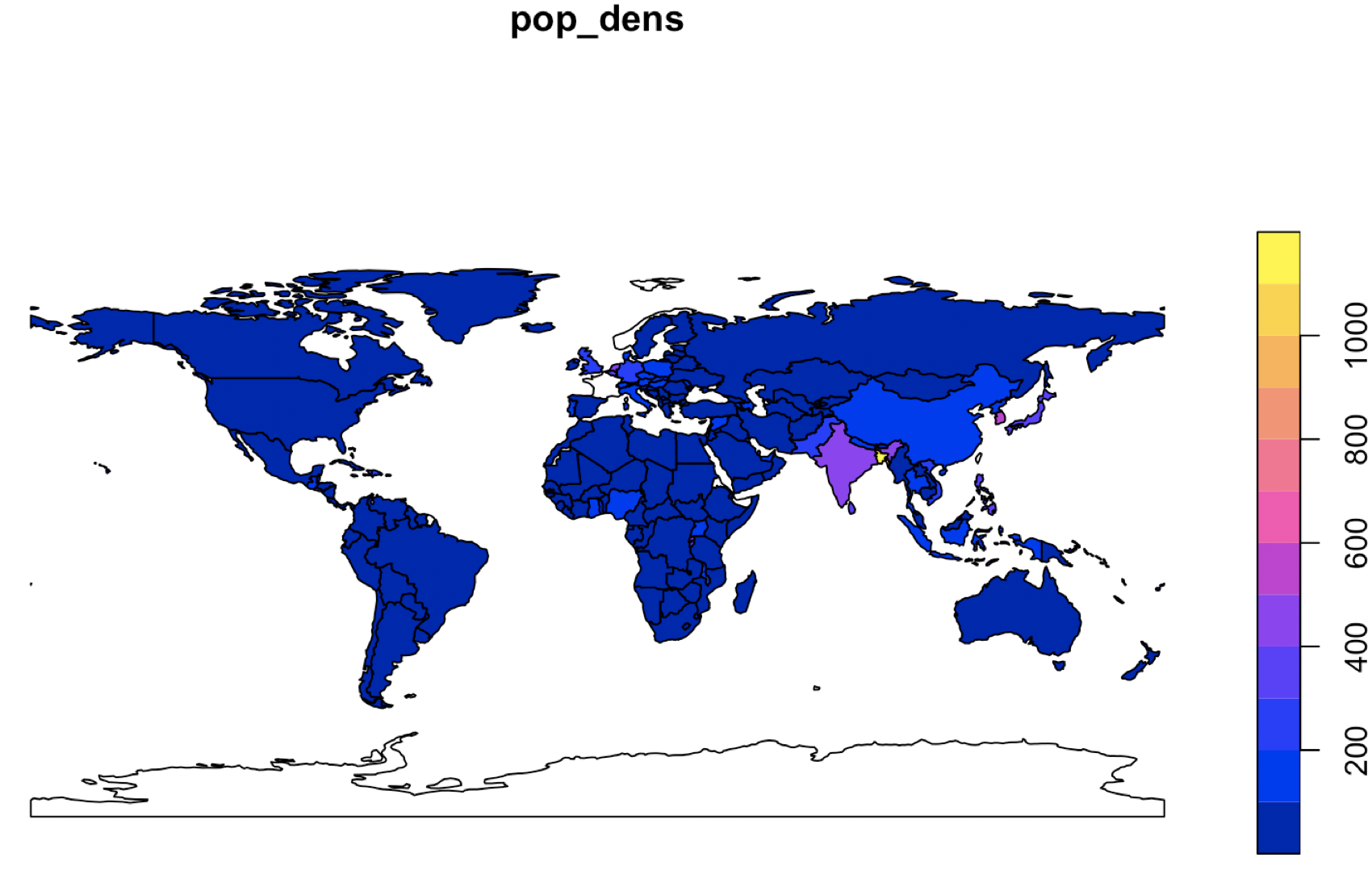
가령, 국가별 인구("pop")를 면적("area_km2")로 나누어서 '(km2 면적 당) 인구밀도("pop_dens")' 라는 새로운 속성을 만들어 보겠습니다. 새로운 속성 칼럼인 "pop_dens"가 생성이 된 후에도 "world_new" 데이터셋은 sf 클래스 객체의 특성을 계속 유지하고 있습니다. 따라서 plot(world_new["pop_dens"] 로 시각화를 하면, 아래와 같이 다면 (multi-polygons) 기하로 표현되는 세계 국가별 지도 위에, 기존 칼럼을 사용해 계산해서 새로 만든 속성 칼럼인 '인구밀도("pop_dens")' 를 시각화할 수 있습니다.
## creating new column using Base R
world_new$pop_dens = world_new$pop / world_new$area_km2


## attribute data operations preserve the geometry of the simple features
## plot() will visualize map using geometry
plot(world_new['pop_dens'])
(2) dplyr 로 지리 벡터 데이터에 새로운 속성 만들기 : mutate(), transmute()
위 (1)번의 Base R 대비 dplyr 를 사용하면, 한꺼번에 여러개의 신규 속성 칼럼을 생성할 수 있고, 체인('%>%')을 이용해서 파이프 연산자로 이전 작업 결과를 다음 작업으로 넘겨주는 방식으로 작업 흐름을 코딩할 수 있어 가독성이 뛰어난 코드를 짤 수 있는 장점이 있습니다.
mutate() 함수는 기존 데이터셋에 새로 만든 데이터셋을 추가해주는 반면에, transmute() 함수는 기존의 칼럼은 모두 제거를 하고 새로 만든 칼럼과 지리기하 geometry 칼럼만을 반환합니다. (이때 sf 클래스 객체의 경우 '지리기하 geometry 칼럼'이 껌딱지처럼 달라붙어서 계속 따라 다닌다는 점이 중요합니다!)
## creating new columns using dplyr
world %>%
  mutate(pop_dens = pop / area_km2)

# Simple feature collection with 177 features and 11 fields
# geometry type:  MULTIPOLYGON
# dimension:      XY
# bbox:           xmin: -180 ymin: -90 xmax: 180 ymax: 83.64513
# geographic CRS: WGS 84
# # A tibble: 177 x 12
# iso_a2 name_long  continent  region_un subregion type  area_km2     pop lifeExp gdpPercap                        geom pop_dens
# * <chr>  <chr>      <chr>      <chr>     <chr>     <chr>    <dbl>   <dbl>   <dbl>     <dbl> <MULTIPOLYGON [arc_degree]>    <dbl>
# 1 FJ     Fiji       Oceania    Oceania   Melanesia Sove~   1.93e4  8.86e5    70.0     8222. (((180 -16.06713, 180 -16.~    45.9
# 2 TZ     Tanzania   Africa     Africa    Eastern ~ Sove~   9.33e5  5.22e7    64.2     2402. (((33.90371 -0.95, 34.0726~    56.0
# 3 EH     Western S~ Africa     Africa    Northern~ Inde~   9.63e4 NA         NA         NA  (((-8.66559 27.65643, -8.6~    NA
# 4 CA     Canada     North Ame~ Americas  Northern~ Sove~   1.00e7  3.55e7    82.0    43079. (((-122.84 49, -122.9742 4~     3.54
# 5 US     United St~ North Ame~ Americas  Northern~ Coun~   9.51e6  3.19e8    78.8    51922. (((-122.84 49, -120 49, -1~    33.5
# 6 KZ     Kazakhstan Asia       Asia      Central ~ Sove~   2.73e6  1.73e7    71.6    23587. (((87.35997 49.21498, 86.5~     6.33
# 7 UZ     Uzbekistan Asia       Asia      Central ~ Sove~   4.61e5  3.08e7    71.0     5371. (((55.96819 41.30864, 55.9~    66.7
# 8 PG     Papua New~ Oceania    Oceania   Melanesia Sove~   4.65e5  7.76e6    65.2     3709. (((141.0002 -2.600151, 142~    16.7
# 9 ID     Indonesia  Asia       Asia      South-Ea~ Sove~   1.82e6  2.55e8    68.9    10003. (((141.0002 -2.600151, 141~   140.
# 10 AR     Argentina  South Ame~ Americas  South Am~ Sove~   2.78e6  4.30e7    76.3    18798. (((-68.63401 -52.63637, -6~    15.4
# # ... with 167 more rows
transmute() 함수를 사용해서 '(km2 면적당) 인구밀도 ("pop_dens")' 의 신규 속성을 만들면, 기존의 속성 칼럼들은 모두 제거 되고 새로운 '인구밀도' 속성 칼럼과 '지리기하 geom' 칼럼만 남게 됩니다.
## -- transmute() drops all other existing columns except for the sticky geometry column
world %>%
  transmute(pop_dens = pop / area_km2)

# Simple feature collection with 177 features and 1 field
# geometry type:  MULTIPOLYGON
# dimension:      XY
# bbox:           xmin: -180 ymin: -90 xmax: 180 ymax: 83.64513
# geographic CRS: WGS 84
# # A tibble: 177 x 2
# pop_dens                                                                                    geom
# *    <dbl>                                                             <MULTIPOLYGON [arc_degree]>
# 1    45.9  (((180 -16.06713, 180 -16.55522, 179.3641 -16.80135, 178.7251 -17.01204, 178.5968 -1...
# 2    56.0  (((33.90371 -0.95, 34.07262 -1.05982, 37.69869 -3.09699, 37.7669 -3.67712, 39.20222 ...
# 3    NA    (((-8.66559 27.65643, -8.665124 27.58948, -8.6844 27.39574, -8.687294 25.88106, -11....
# 4     3.54 (((-122.84 49, -122.9742 49.00254, -124.9102 49.98456, -125.6246 50.41656, -127.4356...
# 5    33.5  (((-122.84 49, -120 49, -117.0312 49, -116.0482 49, -113 49, -110.05 49, -107.05 49,...
# 6     6.33 (((87.35997 49.21498, 86.59878 48.54918, 85.76823 48.45575, 85.72048 47.45297, 85.16...
# 7    66.7  (((55.96819 41.30864, 55.92892 44.99586, 58.50313 45.5868, 58.68999 45.50001, 60.239...
# 8    16.7  (((141.0002 -2.600151, 142.7352 -3.289153, 144.584 -3.861418, 145.2732 -4.373738, 14...
# 9   140.   (((141.0002 -2.600151, 141.0171 -5.859022, 141.0339 -9.117893, 140.1434 -8.297168, 1...
# 10    15.4  (((-68.63401 -52.63637, -68.25 -53.1, -67.75 -53.85, -66.45 -54.45, -65.05 -54.7, -6...
# # ... with 167 more rows
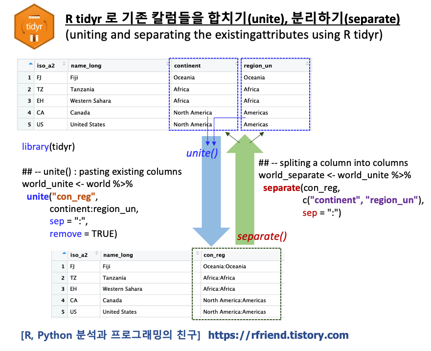
(3) tidyr 로 지리 벡터 데이터의 기존 속성을 합치거나 분리하기 : unite(), separate()
tidyr 패키지에 있는 unite(data, col, lll, sep = "_", remove = TRUE) 함수를 사용하면 기존의 속성 칼럼을 합쳐서 새로운 속성 칼럼을 만들 수 있습니다. 이때 remove = TRUE 매개변수를 설정해주면 기존의 합치려는 두 개의 칼럼은 제거되고, 새로 만들어진 칼럼만 남게 됩니다.
## -- unite(): pasting together existing columns.
library(tidyr)

world_unite = world %>%
  unite("con_reg", continent:region_un,
        sep = ":",
        remove = TRUE)

world_unite
# Simple feature collection with 177 features and 9 fields
# geometry type:  MULTIPOLYGON
# dimension:      XY
# bbox:           xmin: -180 ymin: -90 xmax: 180 ymax: 83.64513
# geographic CRS: WGS 84
# # A tibble: 177 x 10
# iso_a2 name_long   con_reg     subregion    type    area_km2     pop lifeExp gdpPercap                                    geom
# <chr>  <chr>       <chr>       <chr>        <chr>      <dbl>   <dbl>   <dbl>     <dbl>             <MULTIPOLYGON [arc_degree]>
# 1 FJ     Fiji        Oceania:Oc~ Melanesia    Sovere~   1.93e4  8.86e5    70.0     8222. (((180 -16.06713, 180 -16.55522, 179.3~
# 2 TZ     Tanzania    Africa:Afr~ Eastern Afr~ Sovere~   9.33e5  5.22e7    64.2     2402. (((33.90371 -0.95, 34.07262 -1.05982, ~
# 3 EH     Western Sa~ Africa:Afr~ Northern Af~ Indete~   9.63e4 NA         NA         NA  (((-8.66559 27.65643, -8.665124 27.589~
# 4 CA     Canada      North Amer~ Northern Am~ Sovere~   1.00e7  3.55e7    82.0    43079. (((-122.84 49, -122.9742 49.00254, -12~
# 5 US     United Sta~ North Amer~ Northern Am~ Country   9.51e6  3.19e8    78.8    51922. (((-122.84 49, -120 49, -117.0312 49, ~
# 6 KZ     Kazakhstan  Asia:Asia   Central Asia Sovere~   2.73e6  1.73e7    71.6    23587. (((87.35997 49.21498, 86.59878 48.5491~
# 7 UZ     Uzbekistan  Asia:Asia   Central Asia Sovere~   4.61e5  3.08e7    71.0     5371. (((55.96819 41.30864, 55.92892 44.9958~
# 8 PG     Papua New ~ Oceania:Oc~ Melanesia    Sovere~   4.65e5  7.76e6    65.2     3709. (((141.0002 -2.600151, 142.7352 -3.289~
# 9 ID     Indonesia   Asia:Asia   South-Easte~ Sovere~   1.82e6  2.55e8    68.9    10003. (((141.0002 -2.600151, 141.0171 -5.859~
# 10 AR     Argentina   South Amer~ South Ameri~ Sovere~   2.78e6  4.30e7    76.3    18798. (((-68.63401 -52.63637, -68.25 -53.1, ~
# # ... with 167 more rows
tidyr 패키지의 separate(data, col, sep = "[^:alnum:]]+", remove = TRUE, ...) 함수는 기존에 존재하는 칼럼을 구분자(sep)를 기준으로 두 개의 칼럼으로 분리(separation, splitting)를 해줍니다. 이때 remove = TRUE 매개변수를 설정해주면 기존의 분리하려는 원래 속성 칼럼은 제거가 됩니다.
역시, unite() 또는 separate() 함수 적용 후의 결과 데이터셋은 sf 클래스 객체로서, 제일 뒤에 지리기하 geometry 칼럼이 계속 붙어 있습니다.
## -- separate(): splitting one column into multiple columns
## : using either a regular expression or character positions.
world_separate <- world_unite %>%
  separate(con_reg,
           c("continent", "region_un"),
           sep = ":")


world_separate
# Simple feature collection with 177 features and 10 fields
# geometry type:  MULTIPOLYGON
# dimension:      XY
# bbox:           xmin: -180 ymin: -90 xmax: 180 ymax: 83.64513
# geographic CRS: WGS 84
# # A tibble: 177 x 11
#    iso_a2 name_long  continent  region_un subregion   type   area_km2     pop lifeExp gdpPercap                              geom
#    <chr>  <chr>      <chr>      <chr>     <chr>       <chr>     <dbl>   <dbl>   <dbl>     <dbl>       <MULTIPOLYGON [arc_degree]>
#  1 FJ     Fiji       Oceania    Oceania   Melanesia   Sover~   1.93e4  8.86e5    70.0     8222. (((180 -16.06713, 180 -16.55522,~
#  2 TZ     Tanzania   Africa     Africa    Eastern Af~ Sover~   9.33e5  5.22e7    64.2     2402. (((33.90371 -0.95, 34.07262 -1.0~
#  3 EH     Western S~ Africa     Africa    Northern A~ Indet~   9.63e4 NA         NA         NA  (((-8.66559 27.65643, -8.665124 ~
#  4 CA     Canada     North Ame~ Americas  Northern A~ Sover~   1.00e7  3.55e7    82.0    43079. (((-122.84 49, -122.9742 49.0025~
#  5 US     United St~ North Ame~ Americas  Northern A~ Count~   9.51e6  3.19e8    78.8    51922. (((-122.84 49, -120 49, -117.031~
#  6 KZ     Kazakhstan Asia       Asia      Central As~ Sover~   2.73e6  1.73e7    71.6    23587. (((87.35997 49.21498, 86.59878 4~
#  7 UZ     Uzbekistan Asia       Asia      Central As~ Sover~   4.61e5  3.08e7    71.0     5371. (((55.96819 41.30864, 55.92892 4~
#  8 PG     Papua New~ Oceania    Oceania   Melanesia   Sover~   4.65e5  7.76e6    65.2     3709. (((141.0002 -2.600151, 142.7352 ~
#  9 ID     Indonesia  Asia       Asia      South-East~ Sover~   1.82e6  2.55e8    68.9    10003. (((141.0002 -2.600151, 141.0171 ~
# 10 AR     Argentina  South Ame~ Americas  South Amer~ Sover~   2.78e6  4.30e7    76.3    18798. (((-68.63401 -52.63637, -68.25 -~
# # ... with 167 more rows
(4) dplyr 로 지리 벡터 데이터의 속성 이름 바꾸기 : rename(), setNames()
dplyr 패키지로 sf 객체이자 data frame 인 데이터셋의 특정 속성 변수 이름을 바꾸려면 rename(data, new_name = old_name) 함수를 사용합니다.
## -- dplyr::rename()
names(world)
# [1] "iso_a2"    "name_long" "continent" "region_un" "subregion" "type"      "area_km2"  "pop"       "lifeExp"   "gdpPercap"
# [11] "geom"


world_nm <- world %>%
  rename(name = name_long)

names(world_nm)
# [1] "iso_a2"    "name"      "continent" "region_un" "subregion" "type"      "area_km2"  "pop"       "lifeExp"   "gdpPercap"
# [11] "geom"
만약 여러개의 속성 칼럼 이름을 한꺼번에 변경, 혹은 부여하고 싶다면 stats 패키지의 setNames(object = nm, nm) 함수를 dplyr의 체인 파이프 라인에 같이 사용하면 편리합니다.
##-- setNames() changes all column names at once
new_names <- c("i", "n", "c", "r", "s", "t", "a", "p", "l", "gP", "geom")

world_setnm <- world %>%
  setNames(new_names)

names(world_setnm)
# [1] "i"    "n"    "c"    "r"    "s"    "t"    "a"    "p"    "l"    "gP"   "geom"
(5) 지리 벡터 데이터에서 지리 정보 제거하기 : st_drop_geometry()
위의 (1)~(4)번까지의 새로운 속성 칼럼 생성/ 이름 변경 등의 작업을 하고 난 결과 데이터셋에는 항상 '지리기하 geometry' 칼럼이 착 달라붙어서 따라 다녔습니다. 이게 지리공간 데이터 분석을 할 때 '속성(attributes)' 정보와 '지리기하 geometry' 정보를 같이 연계하여 분석해야 하는 경우에는 매우 유용합니다. 하지만, 경우에 따라서는 '속성'정보만 필요하고 '지리기하 geometry' 정보는 필요하지 않을 수도 있을 텐데요, 이럴때 많은 저장 용량과 처리 부하를 차지하는 '지리기하 geometry' 칼럼은 제거하고 싶을 것입니다. 이때 sf 패키지의 st_drop_geometry() 함수를 사용해서 sf 클래스 객체에 들어있는 '지리기하 geometry' 정보를 제거할 수 있습니다.
## -- st_drop_geometry(): remove the geometry

## "sf" class
class(world)
# [1] "sf"         "tbl_df"     "tbl"        "data.frame"

## "data.frame"
world_data <- world %>% st_drop_geometry()
class(world_data)
# [1] "tbl_df"     "tbl"        "data.frame"
[Reference]
[1] Geo-computation with R - Attribute data operations
: geocompr.robinlovelace.net/attr.html
이번 포스팅이 많은 도움이 되었기를 바랍니다.
행복한 데이터 과학자 되세요! :-)