[PyTorch] 텐서 나누기 (splitting a PyTorch tensor into multiple tensors)
Deep Learning (TF, Keras, PyTorch)/PyTorch basics 2023. 2. 23. 00:33지난 포스팅에서는 두 개의 PyTorch 텐서를 합치기 (concatenating two PyTorch tensors) 에 대해서 다루었습니다.
(바로가기 ==> https://rfriend.tistory.com/781 )
이번 포스팅에서는 반대로 한 개의 PyTorch 텐서를 복수 개로 나누기 (splitting a tensor into multiple tensors) 하는 방법을 소개하겠습니다.
(1) 하나의 PyTorch 텐서를 위-아래의 복수 개의 텐서로 나누기
(splitting a tensor into multiple tensors vertically)
: torch.vsplit(tensor, indices_or_sections), torch.split(tensor, split_size_or_sections, dim=0)
(2) 하나의 PyTorch 텐서를 좌-우의 복수 개의 텐서로 나누기
(splitting a tensor into multiple tensors horizontally)
: torch.hsplit(tensor, indices_or_sections), torch.split(tensor, split_size_or_sections, dim=1)
먼저 PyTorch 텐서를 위-아래의 수직으로 복수 개의 텐서로 나누기를 해보겠습니다.
(1) 하나의 PyTorch 텐서를 위-아래의 복수 개의 텐서로 나누기
(splitting a tensor into multiple tensors vertically)
: torch.vsplit(tensor, indices_or_sections), torch.split(tensor, split_size_or_sections, dim=0)
torch.vsplit() 과 torch.split(dim=0) 의 경우 매개변수의 사용법에 차이가 있습니다.
torch.vsplit(tensor, indices_or_sections) 은 indices_or_sections 매개변수로 input tensor 의 행(row) 을 몇으로 나눌지(indices)를, 그래서 결국 몇 개의 텐서로 나누고 싶은지를 지정해주는 것입니다. 가령, 아래 예의 경우 텐서 z 는 Size[6, 6] 인데요, indices_or_sections=2 로 입력할 경우, 6/2 = 3 으로서 각 3개의 균등한 행을 가지는 2개의 텐서로 나누어줍니다.
반면에, torch.split(tensor, split_size_or_sections, dim=0) 은 (a) "dim=0" 으로 행에 대해서 수직으로 텐서 분리를 수행하라고 지정을 해주어야 하고, (b) split_size_or_sections 에서 지정한 숫자만큼의 크기(split_size)로 행을 가지도록 텐서를 분리해줍니다. 가령, 아래 예의 Size[6, 6] 의 텐서 z에 대해서 torch.split(z, 3, dim=0) 으로서 split_size_or_sections = 3 을 입력해주면 각 행을 3개씩의 크기(split size)로 가지는 텐서로 분리를 해줍니다. (원래 텐서에 행이 6개 있는데, 분리할 텐서는 각 3개씩 행을 가지라고 했으므로 결과적으로 총 2개의 텐서로 분리가 됨).

예제로 사용할 Size[6, 6]의 PyTorch 텐서 z 를 만들어보겠습니다.
z = torch.arange(36).reshape(6,6)

print(z)
# tensor([[ 0,  1,  2,  3,  4,  5],
#         [ 6,  7,  8,  9, 10, 11],
#         [12, 13, 14, 15, 16, 17],
#         [18, 19, 20, 21, 22, 23],
#         [24, 25, 26, 27, 28, 29],
#         [30, 31, 32, 33, 34, 35]])
텐서 z 를 torch.vsplit(z, 2) 를 사용해서 2개의 텐서로 분리를 해보겠습니다. (indices_or_sections = 2 로 입력하면 6을 2로 나누어서 3개씩의 행을 가지는 2개의 텐서로 분리해줌)
## vsplit(): Splits input, a tensor with two or more dimensions,
## into multiple tensors vertically according to indices_or_sections.
torch.vsplit(z, 2)

# (tensor([[ 0,  1,  2,  3,  4,  5],
#          [ 6,  7,  8,  9, 10, 11],
#          [12, 13, 14, 15, 16, 17]]),
#  tensor([[18, 19, 20, 21, 22, 23],
#          [24, 25, 26, 27, 28, 29],
#          [30, 31, 32, 33, 34, 35]]))
이때 반환되는 아웃풋은 두 개의 텐서를 묶어놓은 튜플(tuple)입니다.
type(torch.vsplit(z, 2))
# tuple
위에서 2개로 분리한 텐서들의 묶음인 튜플에 원하는 부분의 텐서에 접근하기 위해서는 인덱싱(indexing)을 사용하면 됩니다. 아래 예에서는 2개로 분리한 텐서의 각 첫번째와 두번째 튜플에 접근해서 가져와봤습니다.
## accessing a tensor after splitting
torch.vsplit(z, 2)[0]

# tensor([[ 0,  1,  2,  3,  4,  5],
#         [ 6,  7,  8,  9, 10, 11],
#         [12, 13, 14, 15, 16, 17]])


torch.vsplit(z, 2)[1]

# tensor([[18, 19, 20, 21, 22, 23],
#         [24, 25, 26, 27, 28, 29],
#         [30, 31, 32, 33, 34, 35]])
torch.split(z, 3, dim=0) 은 dim=0 으로 지정을 해주면 됩니다.
## Splits the tensor into chunks.
## Each chunk is a view of the original tensor.
torch.split(z, 3, dim=0)

# (tensor([[ 0,  1,  2,  3,  4,  5],
#          [ 6,  7,  8,  9, 10, 11],
#          [12, 13, 14, 15, 16, 17]]),
#  tensor([[18, 19, 20, 21, 22, 23],
#          [24, 25, 26, 27, 28, 29],
#          [30, 31, 32, 33, 34, 35]]))
## split_size_or_sections : list of sizes for each chunk
torch.split(z, [1,2,3], dim=0)

# (tensor([[0, 1, 2, 3, 4, 5]]),
#  tensor([[ 6,  7,  8,  9, 10, 11],
#          [12, 13, 14, 15, 16, 17]]),
#  tensor([[18, 19, 20, 21, 22, 23],
#          [24, 25, 26, 27, 28, 29],
#          [30, 31, 32, 33, 34, 35]]))
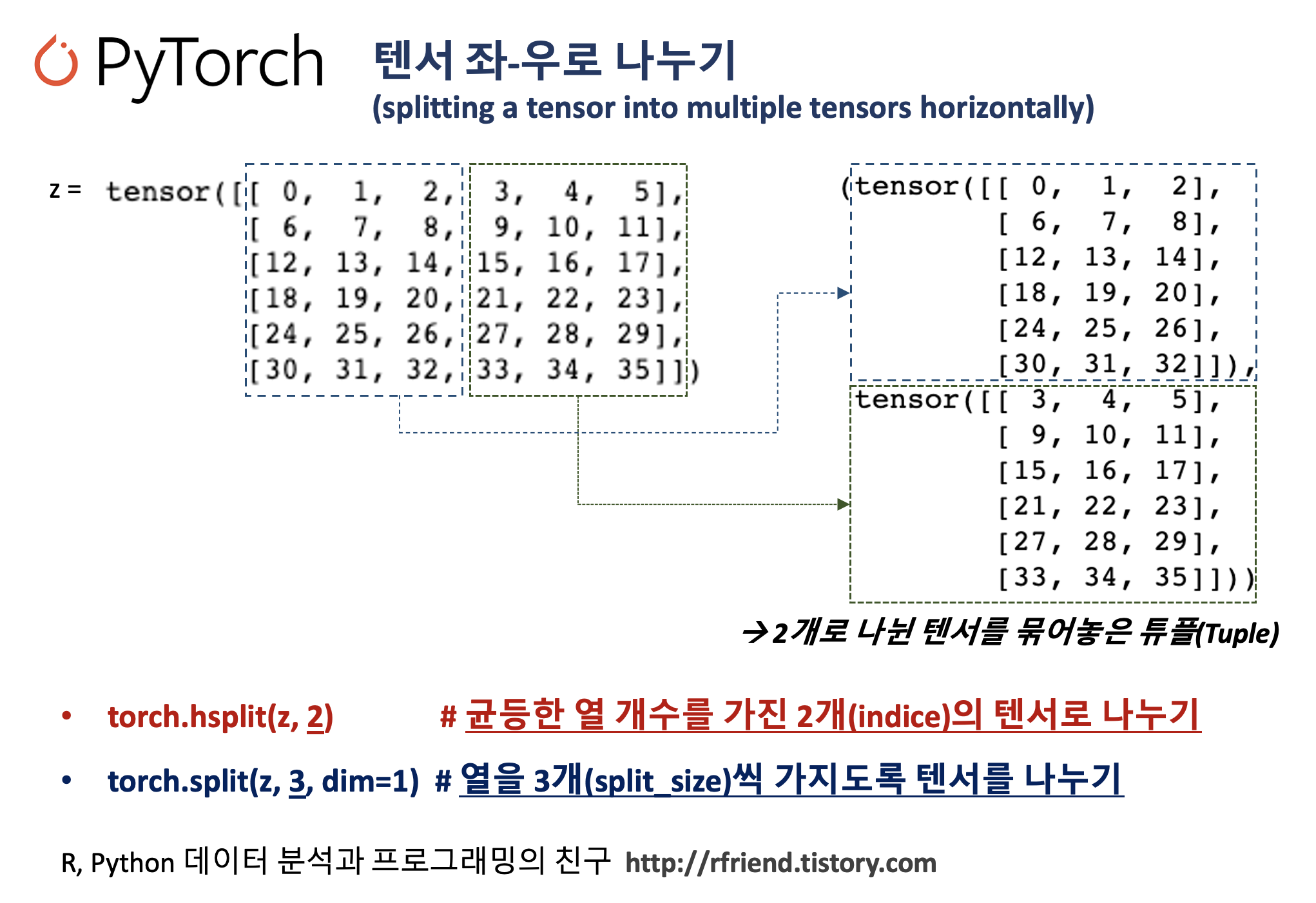
(2) 하나의 PyTorch 텐서를 좌-우의 복수 개의 텐서로 나누기
(splitting a tensor into multiple tensors horizontally)
: torch.hsplit(tensor, indices_or_sections), torch.split(tensor, split_size_or_sections, dim=1)
이번에는 하나의 PyTorch 텐서를 좌-우 수평으로해서 복수 개의 텐서로 나누어볼텐데요, 역시 torch.hsplit() 과 torch.split(dim=1) 의 경우 매개변수의 사용법에 차이가 있습니다.
torch.hsplit(tensor, indices_or_sections) 은 indices_or_sections 매개변수로 input tensor 의 열(column) 을 몇으로 나눌지(indices)를, 그래서 결국 몇 개의 텐서로 나누고 싶은지를 지정해주는 것입니다. 가령, 아래 예의 경우 텐서 z 는 Size[6, 6] 인데요, indices_or_sections=2 로 입력할 경우, 6/2 = 3 으로서 각 3개의 균등한 열을 가지는 2개의 텐서로 좌-우로 나누어줍니다.
반면에, torch.split(tensor, split_size_or_sections, dim=1) 은 (a) "dim=1" 으로 행에 대해서 수평으로 텐서 분리를 수행하라고 지정을 해주어야 하고, (b) split_size_or_sections 에서 지정한 숫자만큼의 크기(split_size)로 행을 가지도록 텐서를 분리해줍니다. 가령, 아래 예의 Size[6, 6] 의 텐서 z에 대해서 torch.split(z, 3, dim=0) 으로서 split_size_or_sections = 3 을 입력해주면 각 열(column)을 3개씩의 크기(split size)로 가지는 텐서로 분리를 해줍니다. (원래 텐서에 열이 6개 있는데, 분리할 텐서는 각 3개씩 열을 가지라고 했으므로 결과적으로 총 2개의 텐서로 분리가 됨).
## hsplit(): Splits input, a tensor with two or more dimensions,
## into multiple tensors horizontally according to indices_or_sections.

torch.hsplit(z, 2)

# (tensor([[ 0,  1,  2],
#          [ 6,  7,  8],
#          [12, 13, 14],
#          [18, 19, 20],
#          [24, 25, 26],
#          [30, 31, 32]]),
#  tensor([[ 3,  4,  5],
#          [ 9, 10, 11],
#          [15, 16, 17],
#          [21, 22, 23],
#          [27, 28, 29],
#          [33, 34, 35]]))
torch.hsplit(tensor, indices_or_sections) 에서 indices_or_sections 매개변수로 indices 넣어줄 때는 정수로 나누어지는 값을 넣어주어야 합니다. 가령, 아래 예에서는 Size[6, 6] 의 텐서에서 dimension 1 의 방향으로 4개 나누라고 지정해었더닌 6을 4로 나눌 수 없다면서 RunTimeError: torch.hsplit attempted to split along dimension 1, but size of the dimension 6 is not divisible by the split_size 4! 라는 에러가 발생했습니다.
## RuntimeError
torch.hsplit(z, 4)

# RuntimeError: torch.hsplit attempted to split along dimension 1,
# but the size of the dimension 6 is not divisible by the split_size 4!
torch.split(z, 3, dim=1) 에서는 dim=1 로 차원을 지정해주면 됩니다.
torch.split(z, 3, dim=1)

# (tensor([[ 0,  1,  2],
#          [ 6,  7,  8],
#          [12, 13, 14],
#          [18, 19, 20],
#          [24, 25, 26],
#          [30, 31, 32]]),
#  tensor([[ 3,  4,  5],
#          [ 9, 10, 11],
#          [15, 16, 17],
#          [21, 22, 23],
#          [27, 28, 29],
#          [33, 34, 35]]))
torch.split() 함수에서 split_size_or_sections 매개변수에 리스트로 해서 나누고 싶은 텐서의 크기 (split_size_sections) 를 복수개로 지정해줄 수도 있습니다. 아래의 예에서는 Size[6, 6]의 텐서를 열의 개수를 1개, 2개, 3개를 가지는 총 3개의 텐서로 분리(split_size_or_sections = [1, 2, 3])해 본 것입니다. 매우 편리한 기능입니다!
## split_size_or_sections : list of sizes for each chunk
torch.split(z, [1,2,3], dim=1)

# (tensor([[ 0],
#          [ 6],
#          [12],
#          [18],
#          [24],
#          [30]]),
#  tensor([[ 1,  2],
#          [ 7,  8],
#          [13, 14],
#          [19, 20],
#          [25, 26],
#          [31, 32]]),
#  tensor([[ 3,  4,  5],
#          [ 9, 10, 11],
#          [15, 16, 17],
#          [21, 22, 23],
#          [27, 28, 29],
#          [33, 34, 35]]))
이번 포스팅이 많은 도움이 되었기를 바랍니다.
행복한 데이터 과학자 되세요! :-)

'Deep Learning (TF, Keras, PyTorch) > PyTorch basics' 카테고리의 다른 글
| 딥러닝에서 오차역전파법 (Backpropagation, Backward Propagation of Errors) 이란? (0) | 2023.12.12 |
|---|---|
| [PyTorch] torchvision.datasets 모듈에 내장되어 있는 데이터 가져와서 시각화하기 (0) | 2023.02.26 |
| [PyTorch] 텐서 합치기 (concat, stack) (0) | 2023.02.21 |
| [PyTorch] 텐서의 인덱싱과 슬라이싱 (indexing & slicing of PyTorch tensor) (0) | 2023.02.19 |
| [PyTorch] NumPy의 array 대비 PyTorch 의 성능 비교 (0) | 2023.02.19 |

 abalone.txt


