이번 포스팅에서는 Python pandas 의 DataFrame에서 문자열(string)을 데이터 형태로 가지는 칼럼을 특정 기준(separator, delimiter) 분할(split a string)하여, 그 중의 일부분을 가져다가 DataFrame에 새로운 칼럼으로 만들어서 붙이는 2가지 방법을 소개하겠습니다. 


(1) Vectorization을 이용한 pandas DataFrame 문자열 칼럼 분할하기

(2) For Loop operation을 통한 pandas DataFrame 문자열 칼럼 분할하기


Python pandas DataFrame: Split string column and make a new column using part of it.


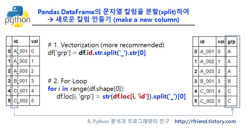
(1) Vectorization을 이용한 pandas DataFrame 문자열 칼럼 분할하기 (빠름 ^^)


예제로 사용할 문자열 'id' 와 숫자형 'val' 의 두 개 칼럼으로 이루어진 DataFrame을 만들어보겠습니다. 그리고 문자열 'id' 칼럼을 구분자(separator) '_' 를 기준으로 str.split('_') 메소드를 사용하여 분할(split) 한 후에, 앞부분([0])을 가져다가 'grp'라는 칼럼을 추가하여 만들어보겠습니다. 


import numpy as np
import pandas as pd


df = pd.DataFrame({'id': ['A_001', 'A_002', 'A_003', 'B_001', 'C_001', 'C_002'], 
                          'val': np.arange(6)})


print(df)

   id       val

0 A_001  0

1 A_002  1

2 A_003  2

3 B_001  3

4 C_001  4

5 C_002  5


# 1. vectorization
df['grp'] = df.id.str.split('_').str[0]

print(df)

   id       val  grp

0 A_001  0    A

1 A_002  1    A

2 A_003  2    A

3 B_001  3    B

4 C_001  4    C

5 C_002  5    C


만약 리스트(list)로 만들고 싶으면 분할한 객체에 대해 tolist() 메소드를 사용하면 됩니다. 

# tolist()
grp_list = df.id.str.split('_').str[0].tolist()
print(grp_list)

['A', 'A', 'A', 'B', 'C', 'C']


(2) For Loop operation을 통한 pandas DataFrame 문자열 칼럼 분할하기 (느림 -_-;;;)


두번째는 For Loop 연산을 사용하여 한 행, 한 행씩(row by row) 분할하고, 앞 부분 가져다가 'grp' 칼럼에 채워넣고... 를 반복하는 방법입니다. 위의 (1)번의 한꺼번에 처리하는 vectorization 대비 (2)번의 for loop은 시간이 상대적으로 많이 걸립니다. 데이터셋이 작으면 티가 잘 안나는데요, 수백~수천만건이 되는 자료에서 하면 느린 티가 많이 납니다. 


# 2. for loop
df = pd.DataFrame({'id': ['A_001', 'A_002', 'A_003', 'B_001', 'C_001', 'C_002'], 
                  'val': np.arange(6)})


for i in range(df.shape[0]):
    df.loc[i, 'grp'] = str(df.loc[i, 'id']).split('_')[0]


print(df)

   id       val  grp

0 A_001  0    A

1 A_002  1    A

2 A_003  2    A

3 B_001  3    B

4 C_001  4    C

5 C_002  5    C


많은 도움이 되었기를 바랍니다.

728x90
반응형
Posted by Rfriend
,

이번 포스팅에서는 다수 그룹 별 다수의 변수 간 쌍을 이룬 상관계수 분석(paired correlation coefficients with multiple columns by multiple groups) 을 하는 방법을 소개하겠습니다. 


보통 다수의 변수간의 상관계수를 구할 때는 상관계수 행렬 (correlation matrix)를 하면 되는데요, 이때 '다수의 그룹별 (by multiple groups)'로 나누어서 다수의 변수 간 상관계수를 구하려면 머리가 좀 복잡해집니다. 


간단한 예제 데이터셋을 만들어서 예를 들어보겠습니다. 


(1) 3개의 그룹 변수, 4개의 연속형 변수를 가진 예제 DataFrame 만들기


import numpy as np

import pandas as pd


'group_1' 변수 내 ('A', 'B' 그룹), 'group_2' 변수 내 ('C', 'D', 'E', 'F' 그룹), 'group_3' 변수 내 ('G', 'H', 'I', 'J', 'K', 'L', 'M', 'N' 그룹) 별로 나누어서 상관계수를 구해보겠습니다.  


# making groups

group_1 = ['A', 'B']*20

group_2 = ['C', 'D', 'E', 'F']*10

group_3 = ['G', 'H', 'I', 'J', 'K', 'L', 'M', 'N']*5;


상관계수를 구할 연속형 변수는 'col_1', 'col_2', 'col_3', 'col_4' 라는 4개의 변수를 사용하겠습니다. 


df = pd.DataFrame({'group_1': group_1, 

                   'group_2': group_2,

                   'group_3': group_3,

                   'col_1': np.random.randn(40), 

                   'col_2': np.random.randn(40), 

                   'col_3': np.random.randn(40), 

                   'col_4': np.random.randn(40)})


df.sort_values(by=['group_1', 'group_2', 'group_3'], axis=0)

col_1col_2col_3col_4group_1group_2group_3
0-0.3519690.026318-1.0379100.849338ACG
8-0.163435-0.175277-1.3492510.645246ACG
160.7286521.7317620.691091-0.189488ACG
24-1.4909560.083991-0.5037271.690979ACG
320.0763800.634184-0.424101-0.608869ACG
40.9020271.454501-1.4678170.448042ACK
120.8997920.8332890.829877-0.062950ACK
20-0.5599710.5399670.0053970.362061ACK
28-1.0525390.558581-0.7993140.979169ACK
360.919377-1.430321-1.8183650.061561ACK
2-0.030675-0.168537-1.341236-1.149740AEI
100.112267-0.4767360.967436-0.222528AEI
18-0.774158-0.0812310.4385141.611915AEI
26-0.173712-1.3584140.6533920.053665AEI
341.1100801.175692-0.8678431.042837AEI
6-0.083481-0.200750-0.702476-1.072645AEM
140.223843-1.3453150.8996681.126941AEM
220.5296800.0627431.035399-0.729469AEM
301.456441-0.403748-0.4460940.408010AEM
38-1.3085480.367232-0.9631090.918776AEM
10.579627-1.720893-0.798200-0.107270BDH
92.101038-0.581516-0.7962300.324806BDH
17-0.168765-1.176664-0.024593-0.348601BDH
250.166594-1.4183070.916661-0.912822BDH
330.8896150.014690-0.7114580.649833BDH
51.1998020.968027-0.7804340.884857BDL
13-0.0386370.6947500.219160-0.693826BDL
21-1.054844-0.559508-0.890659-0.321867BDL
29-0.5748880.812719-0.823804-0.382432BDL
370.6705480.1789110.497704-0.402953BDL
30.477194-0.355853-1.4418981.418857BFJ
110.9651870.5630260.964660-0.249644BFJ
19-2.3186850.079057-0.107432-1.358502BFJ
27-0.951459-0.4669331.141424-2.860606BFJ
35-0.462823-0.3970810.373452-1.303045BFJ
70.398693-0.086113-0.0814450.871010BFN
150.1219700.2581300.654156-0.497327BFN
231.228697-0.625133-1.761145-0.577502BFN
311.0748550.7841400.5291900.479893BFN
390.3417670.170529-0.2878840.329371BFN


  (2) 그룹별 두 개 변수 간 상관계수를 구하는 사용자 정의 함수


예제 데이터셋이 준비가 되었으니 이제 '그룹별로 두 개 변수 간 상관계수를 구하는 사용자 정의 함수 (a user-defined function of correlation coefficients with paired variables by groups)' 를 정의해보겠습니다. 


# a user-defined function of correlation coefficients with paired variables by groups

def corr_group(df, var_1, var_2, group_list):

    # correlaiton fuction with 2 variables

    corr_func = lambda g: g[var_1].corr(g[var_2])


    # GroupBy operator

    grouped = df.groupby(group_list)


    # calculate correlation coefficient by Group

    corr_coef_df = pd.DataFrame(grouped.apply(corr_func), columns=['corr_coef'])


    # add var_1, var_2 column names

    corr_coef_df['var1'] = var_1

    corr_coef_df['var2'] = var_2


    return corr_coef_df


  (3) 다수 그룹별 다수 변수 간 두개 씩 쌍을 이루어 상관계수 구하기


'group_1', 'group_2', 'group_3' 의 3개의 그룹 변수로 만들어진 모든 경우의 수의 그룹 조합에 대해서, 'col_1', 'col_2', 'col_3', 'col_4'의 4개 연속형 변수로 2개씩 쌍(pair)을 이루어 만들어진 모든 경우의 수의 조합, 즉, ('col_1', 'col_2'), ('col_1', 'col_3'), ('col_1', 'col_4'), ('col_2', 'col_3'), ('col_2', 'col_4'), ('col_3', 'col_4') 의 4C2=6개의 조합별 상관계수를 구해보겠습니다. 


이때 위의 (2)번에서 만들었던 '두 개 쌍의 변수간 상관계수 구하는 사용자 정의함수'인 corr_group() 함수를 사용하여 for loop 문으로 6개의 연속형 변수의 조합별로 상관계수를 구한 후에, corr_coef_df_all 데이터 프레임에 append 해나가는 방식을 사용하였습니다. 


# blank DataFrame

corr_coef_df_all = pd.DataFrame()


# group by list

group_list = ['group_1', 'group_2', 'group_3']


# column lists for correlation matrix

col_list = ['col_1', 'col_2', 'col_3', 'col_4']


# get all cominations of col_list with length 2

from itertools import combinations

comb = combinations(col_list, 2)


# calculate correlation coefficients pair-wise

for var in list(comb):

    corr_tmp = corr_group(df, var[0], var[1], group_list)

    corr_coef_df_all = corr_coef_df_all.append(corr_tmp)


# result

corr_coef_df_all[['var1', 'var2', 'corr_coef']]

var1var2corr_coef
group_1group_2group_3
ACGcol_1col_20.703392
Kcol_1col_2-0.139566
EIcol_1col_20.642818
Mcol_1col_2-0.410050
BDHcol_1col_20.511432
Lcol_1col_20.569900
FJcol_1col_20.247295
Ncol_1col_2-0.186798
ACGcol_1col_30.466368
Kcol_1col_3-0.167176
EIcol_1col_3-0.455445
Mcol_1col_30.385438
BDHcol_1col_3-0.615976
Lcol_1col_30.362789
FJcol_1col_3-0.063979
Ncol_1col_3-0.556404
ACGcol_1col_4-0.867131
Kcol_1col_4-0.790912
EIcol_1col_4-0.052166
Mcol_1col_4-0.191858
BDHcol_1col_40.656101
Lcol_1col_40.631548
FJcol_1col_40.604571
Ncol_1col_4-0.144041
ACGcol_2col_30.956775
Kcol_2col_30.423775
EIcol_2col_3-0.597295
Mcol_2col_3-0.506746
BDHcol_2col_3-0.399239
Lcol_2col_30.036270
FJcol_2col_30.262685
Ncol_2col_30.875746
ACGcol_2col_4-0.631931
Kcol_2col_40.315081
EIcol_2col_40.395802
Mcol_2col_4-0.381141
BDHcol_2col_40.789146
Lcol_2col_40.363601
FJcol_2col_40.216682
Ncol_2col_40.406150
ACGcol_3col_4-0.434402
Kcol_3col_4-0.250838
EIcol_3col_40.274027
Mcol_3col_4-0.008633
BDHcol_3col_4-0.874220
Lcol_3col_4-0.472953
FJcol_3col_4-0.775485
Ncol_3col_40.366142


많은 도움이 되었기를 바랍니다. 


이번 포스팅이 도움이 되었다면 아래의 '공감~'를 꾹 눌러주세요. :-)


728x90
반응형
Posted by Rfriend
,

이번 포스팅은 두 개의 연속형 변수에 대한 관계를 파악하는데 유용하게 사용할 수 있는 산점도(Scatter Plot) 의 세번째 포스팅으로서 4개의 연속형 변수를 사용하여 X축, Y축, 점의 색깔(color)과 크기(size)을 다르게 하는 방법을 소개합니다. 


즉, 산점도를 사용하여 4차원의 데이터를 2차원에 시각화하는 방법입니다. 


(1) 산점도 (Scatter Plot)

(2) 그룹별 산점도 (Scatter Plot by Groups)

(3) 4개 변수로 점의 크기와 색을 다르게 산점도 그리기 (Scatter plot with different size, color)

(4) 산점도 행렬 (Scatter Plot Matrix)


예제로 활용할 데이터는 iris 의 4개의 연속형 변수들입니다. 


# importing libraries

import numpy as np

import pandas as pd


import matplotlib.pyplot as plt

import seaborn as sns

plt.rcParams['figure.figsize'] = [10, 8] # setting figure size


# loading 'iris' dataset from seaborn

iris = sns.load_dataset('iris')

iris.shape

(150, 5)


iris.head()

sepal_lengthsepal_widthpetal_lengthpetal_widthspecies
05.13.51.40.2setosa
14.93.01.40.2setosa
24.73.21.30.2setosa
34.63.11.50.2setosa
45.03.61.40.2setosa


  (1) matplotlib에 의한 4개 연속형 변수를 사용한 산점도 (X축, Y축, 색, 크기)


plt.scatter() 함수를 사용하며, 점의 크기는 s, 점의 색깔은 c 에 변수를 할당해주면 됩니다. 


# 4 dimensional scatter plot with different size & color

plt.scatter(iris.sepal_length, # x

           iris.sepal_width, # y

           alpha=0.2, 

           s=200*iris.petal_width, # marker size

           c=iris.petal_length, # marker color

           cmap='viridis')

plt.title('Scatter Plot with Size(Petal Width) & Color(Petal Length)', fontsize=14)

plt.xlabel('Sepal Length', fontsize=12)

plt.ylabel('Sepal Width', fontsize=12)

plt.colorbar()

plt.show()


점(marker)의 모양을 네모로 바꾸고 싶으면 marker='s' 로 설정해주면 됩니다. 


# 4 dimensional scatter plot with different size & color

plt.scatter(iris.sepal_length, # x

           iris.sepal_width, # y

           alpha=0.2, 

           s=200*iris.petal_width, # marker size

           c=iris.petal_length, # marker color

           cmap='viridis'

           marker = 's') # square shape

plt.title('Size(Petal Width) & Color(Petal Length) with Square Marker', fontsize=14)

plt.xlabel('Sepal Length', fontsize=12)

plt.ylabel('Sepal Width', fontsize=12)

plt.colorbar()

plt.show()


  (2) seaborn에 의한 4개 연속형 변수를 사용한 산점도 (X축, Y축, 색, 크기)


seaborn 의 산점도 코드는 깔끔하고 이해하기에 쉬으며, 범례도 잘 알아서 색깔과 크기를 표시해주는지라 무척 편리합니다. 


# 4 dimensional scatter plot by seaborn

sns.scatterplot(x='sepal_length', 

                y='sepal_width', 

                hue='petal_length',

                size='petal_width',

                data=iris)

plt.show()


  (3) pandas에 의한 4개 연속형 변수를 사용한 산점도 (X축, Y축, 색, 크기)


pandas의 DataFrame에 plot(kind='scatter') 로 해서 color=iris['petal_length']로 색깔을 설정, s=iris['petal_width'] 로 크기를 설정해주면 됩니다. pandas 산점도 코드도 깔끔하고 이해하기 쉽긴 한데요, 범례 추가하기가 쉽지가 않군요. ^^; 


iris.plot(kind='scatter'

          x='sepal_length', 

          y='sepal_width', 

          color=iris['petal_length'],

          s=iris['petal_width']*100)


plt.title('Size(Petal Width) & Color(Petal Length) with Square Marker', fontsize=14)

plt.show()


참고로, 산점도의 점(marker)의 모양(shape)을 설정하는 심벌들은 아래와 같으니 참고하시기 바랍니다. 


# set the size

plt.rcParams['figure.figsize'] = [10, 8]


# remove ticks and values of axis

plt.xticks([])

plt.yticks([])


# markers' shape

all_shape=['.','o','v','^','>','<','s','p','*','h','H','D', 'd', '', '', '']


num = 0

for x in range(1, 5):

    for y in range(1, 5):

        num += 1


        plt.plot(x, y, 

                 marker = all_shape[num-1], 

                 markerfacecolor='green', 

                 markersize=20, 

                 markeredgecolor='black')


        plt.text(x+0.1, y, 

                 all_shape[num-1], 

                 horizontalalignment='left', 

                 size='medium', 

                 color='black', 

                 weight='semibold')


plt.title('Markers', fontsize=20)        

plt.show()


많은 도움이 되었기를 바랍니다. 


이번 포스팅이 도움이 되었다면 아래의 '공감~'를 꾹 눌러주세요. ^^


다음번 포스팅에서는 산점도 행렬 (Scatter Plot Matrix) 에 대해서 소개하겠습니다. 


728x90
반응형
Posted by Rfriend
,

이번 포스팅에서는 Python pandas의 GroupBy()와 apply() 함수를 사용하여 그룹별로 무작위 표본 추출 (Random Sampling and Permutation by Groups) 하는 방법을 소개하겠습니다. 


무작위 표본 추출을 하는 데는 np.random.permutation() 함수를 사용해서 순열을 무작위로 뒤섞은 후에 n개 만큼 indexing 해오는 방법을 사용하였습니다. 


[ 그룹 별 무작위 표본 추출 (Random Sampling and Permutation by Groups) ]


먼저 예제로 사용한 'grp_1'과 'grp_2'의 두 개의 그룹을 포함한 DataFrame을 만들어보겠습니다. 


import numpy as np

import pandas as pd


# setting seed number for reproducibility

np.random.seed(123)


# Make a DataFrame

df = pd.DataFrame({'grp': ['grp_1']*10 + ['grp_2']*10, 

                          'col_1': np.random.randint(20, size=20), 

                          'col_2': np.random.randint(20, size=20)})


df

col_1col_2grp
01316grp_1
124grp_1
2217grp_1
363grp_1
4172grp_1
5197grp_1
6102grp_1
7115grp_1
8016grp_1
9177grp_1
10159grp_2
1193grp_2
1206grp_2
13141grp_2
1402grp_2
15151grp_2
161912grp_2
17148grp_2
1843grp_2
19010grp_2


사용자가 지정한 샘플링 비율(sample_pct) 만큼 무작위 표본 추출을 해주는 사용자 정의 함수 (User Defined Function)을 정의해보겠습니다. 


# UDF of random sampling

def sampling_func(data, sample_pct):

    np.random.seed(123)

    N = len(data)

    sample_n = int(len(data)*sample_pct) # integer

    sample = data.take(np.random.permutation(N)[:sample_n])

    return sample


이제 위의 무작위 샘플링 사용자 정의 함수(UDF)를 GroupBy()와 apply() 함수에 적용해서 그룹별 특정 비율(이 예에서는 80%)만큼 무작위 표본 추출(random sampling and permutation by groups)을 해보겠습니다.  


# Apply random sampling UDF to groups

sample_set = df.groupby('grp').apply(sampling_func, sample_pct=0.8)


sample_set.sort_index()

col_1col_2grp
grp
grp_101316grp_1
124grp_1
363grp_1
4172grp_1
5197grp_1
6102grp_1
7115grp_1
8016grp_1
grp_210159grp_2
1193grp_2
13141grp_2
1402grp_2
15151grp_2
161912grp_2
17148grp_2
1843grp_2


위의 무작위 표본 추출 결과에서 group_keys 를 없애려면 group_keys = False 를 지정해주면 됩니다. 


# disable group_keys

sample_set = df.groupby('grp', group_keys=False).apply(sampling_func, sample_pct=0.8)


sample_set.sort_index()

col_1col_2grp
01316grp_1
124grp_1
363grp_1
4172grp_1
5197grp_1
6102grp_1
7115grp_1
8016grp_1
10159grp_2
1193grp_2
13141grp_2
1402grp_2
15151grp_2
161912grp_2
17148grp_2
1843grp_2


위의 80% 무작위 샘플링이 된 sample_set 에 있는 데이터셋을 training_set 이라고 가정해보고, 위의 sample_set에는 없지만 원래 데이터에는 있던 나머지 20% 데이터를 test_set 으로 별도로 만들어보겠습니다. 


test_set = df.drop(df.index[sample_set.index])

test_set

col_1col_2grp
2217grp_1
9177grp_1
1206grp_2
19010grp_2


참고로, pandas DataFrame에 대한 무작위 표본 추출 방법은 https://rfriend.tistory.com/602 를 참고하세요.


많은 도움이 되었기를 바랍니다. 


이번 포스팅이 도움이 되었다면 아래의 '공감~'를 꾹 눌러주세요. ^^


728x90
반응형
Posted by Rfriend
,

여러번에 걸친 지난 포스팅에서는 groupby()와 apply()를 이용하여 그룹 별로 통계량을 구한다든지, 결측값을 대체한다든지, 변수 간 상관계수를 구하는 방법을 소개하였습니다.  


이번 포스팅에서는 groupby()와 apply()를 사용하여 그룹 별로 선회회귀모형을 적합(Group-wise Linear Regression)하는 방법을 소개하겠습니다. 


그룹 개수가 많고, 그룹별로 회귀계수를 비교하고자 할 때 이번 포스팅을 참고하면 그룹별로 일일이 하나씩 모형을 적합하지 않고도 짧은 코드로 간편하게 그룹별 회귀모형을 적합할 수 있습니다. 


[ 그룹 별 선형회귀모형 적합 (Group-wise Linear Regression) ]


예제에 사용할 diabetes (당뇨병) 데이터와 선형회귀모형을 적합할 때 사용할 sklearn의 linear_model 모듈을 importing 하겠습니다. 


당뇨병 환자 442명의 'age', 'sex', bmi', bp', 's1', 's2', 's3', 's4', 's5', 's6' 등의 10개 설명변수와, 우리가 예측하고자 하는 'target' 반응변수가 있는 데이터셋입니다. 설명변수는 표준화가 되어있군요. 


import numpy as np

import pandas as pd

from sklearn import datasets, linear_model


diabetes = datasets.load_diabetes()


diabetes.DESCR 

'Diabetes dataset
================
Notes
-----
Ten baseline variables, age, sex, body mass index, average blood

npressure, and six blood serum measurements were obtained for each of n =442 diabetes patients, as well as the response of interest, a\nquantitative measure of disease progression one year after baseline.\n\nData Set Characteristics:\n\n :Number of Instances: 442\n\n :Number of Attributes: First 10 columns are numeric predictive values\n\n :Target: Column 11 is a quantitative measure of disease progression one year after baseline\n\n :Attributes:\n :Age:\n :Sex:\n :Body mass index:\n :Average blood pressure:\n :S1:\n :S2:\n :S3:\n :S4:\n :S5:\n :S6:\n\nNote: Each of these 10 feature variables have been mean centered and scaled by the standard deviation times `n_samples` (i.e. the sum of squares of each column totals 1).\n\nSource URL:\nhttp://www4.stat.ncsu.edu/~boos/var.select/diabetes.html\n\nFor more information see:\nBradley Efron, Trevor Hastie, Iain Johnstone and Robert Tibshirani (2004) "Least Angle Regression," Annals of Statistics (with discussion), 407-499.\n(http://web.stanford.edu/~hastie/Papers/LARS/LeastAngle_2002.pdf)\n'


diabetes.feature_names

['age', 'sex', 'bmi', 'bp', 's1', 's2', 's3', 's4', 's5', 's6']

diabetes.target[:5]
array([151.,  75., 141., 206., 135.])


이번 포스팅이 '그룹'별 선형회귀모형 분석이므로 'sex(성별)'을 'M (Male)', 'F (Female)' 의 2개 그룹으로 나누어서 'age', 'bmi' 의 2개의 설명변수만을 사용하여 'target' 을 예측하는 그룹별 회귀모형을 적합하여 보겠습니다. 필요한 변수만 선별해서 DataFrame을 만들어보겠습니다. 


# Make a DataFrame of Y ('target')

diabetes_Y = pd.DataFrame(diabetes.target, columns = ['target'])

diabetes_Y[:5]

target
0151.0
175.0
2141.0
3206.0
4135.0


# Make a DataFrame of X with age, sex, bmi

diabetes_X = pd.DataFrame(diabetes.data[:, 0:3], 

                          columns = ['age', 'sex', 'bmi']) # age, sex, bmi


diabetes_X[:5]

agesexbmi
00.0380760.0506800.061696
1-0.001882-0.044642-0.051474
20.0852990.0506800.044451
3-0.089063-0.044642-0.011595
40.005383-0.044642-0.036385


diabetes_df = pd.concat([diabetes_Y, diabetes_X], axis=1)

diabetes_df[:5]

targetagesexbmi
0151.00.0380760.0506800.061696
175.0-0.001882-0.044642-0.051474
2141.00.0852990.0506800.044451
3206.0-0.089063-0.044642-0.011595
4135.00.005383-0.044642-0.036385


'sex' 변수를 가지고 'M', 'F' 를 class로 가지는 'grp'라는 범주형 변수를 만든 후에, 'sex' 변수는 삭제하겠습니다. 


diabetes_df['grp'] = np.where(diabetes_df['sex'] > 0, 'M', 'F')

diabetes_df.drop(columns=['sex'], inplace=True) 

diabetes_df[:3]

targetagebmigrp
0151.00.0380760.061696M
175.0-0.001882-0.051474F
2141.00.0852990.044451M


이제 GroupBy()의 apply()에 사용할 선형회귀모형 사용자 정의 함수(UDF)를 정의해보겠습니다. 각 그룹별 age와 bmi변수의 회귀계수를 비교하고 싶다고 했으므로 사용자 정의 함수에서 그룹별 회귀모형의 회귀계수와 절편을 결과로 반환하도록 하였습니다. 


# UDF of linear regression model

def lin_regress(data, yvar, xvars):


    # output, input variables

    Y = data[yvar]

    X = data[xvars]


    # Create linear regression object

    linreg = linear_model.LinearRegression()


    # Fit the linear regression model

    model = linreg.fit(X, Y)


    # Get the intercept and coefficients

    intercept = model.intercept_

    coef = model.coef_

    result = [intercept, coef]


    return result


다음으로 GroupBy()와 apply()를 사용해서 성별 그룹('M', 'F')별 선형회귀모형을 적합해보겠습니다. 


# GroupBy

grouped = diabetes_df.groupby('grp')

# Apply the UDF of linear regression model by Group

lin_reg_coef = grouped.apply(lin_regress, 'target', ['age', 'bmi'])


남성('M')과 여성('F') 그룹별 Y절편과 age, bmi 변수의 회귀계수 적합 결과를 조회해보겠습니다. 


lin_reg_coef

grp
F    [152.40684676047456, [23.199210147823813, 814....
M    [148.21507864445124, [291.7563226838977, 1092.... 

dtype: object 


lin_reg_coef['M']

[148.21507864445124, array([ 291.75632268, 1092.80118705])]


lin_reg_coef['F']

[152.40684676047456, array([ 23.19921015, 814.50932703])]


위의 그룹별 선형회귀무형 적합 결과로부터 우리는 아래의 모형을 얻었습니다. 

  • 남성('M') 그룹의 당뇨병 진단 target = 148.2 + 291.8*age + 1,092.8*bmi
  • 여성('F') 그룹의 당뇨병 진단 target = 152.4 + 23.2*age + 814.5*bmi

(이때 age, bmi 는 표준화한 후의 input 값임)


따라서 다른 변수가 고정되었다고 했을 때 (표준화한) bmi 값이 한 단위 증가할 때 '남성('M')' 그룹의 당뇨병 진단 target 은 1,092.8 만큼 증가하는 반면에 '여성('F') 그룹의 당뇨병 진단 target은 814.5 만큼 증가하는 것으로 나왔습니다. 


많은 도움이 되었기를 바랍니다. 


이번 포스팅이 도움이 되었다면 아래의 '공감~'를 꾹 눌러주세요. ^^


728x90
반응형
Posted by Rfriend
,

이번 포스팅에서는 그룹 별로 변수 간 상관관계 분석 (correlation with columns by groups) 하는 방법을 소개하겠습니다. 


Python pandas는 Pearson Correlation Coefficient를 구할 수 있는 corr(), corrwith() 함수를 제공합니다. 이들 함수를 groupby() 와 apply(lambda func)를 함께 사용함으로써 그룹 별 변수 간 상관계수를 구할 수 있습니다. 


[ 피어슨 상관계수 ( Pearson Correlation Coefficient) ]


먼저 예제로 사용할 'group 1'과 'group 2'의 2개의 그룹을 가진 간단한 DataFrame을 만들어보겠습니다. 


import numpy as np

import pandas as pd

from pandas import DataFrame


# making DataFrame with 4 random variables

np.random.seed(123) # for reproducibility

df= DataFrame(np.random.randn(10, 4), 

                    columns=['a', 'b', 'c', 'd'])

# setting index with 2 group, 'grp1' and 'grp2'

df['group'] = ['grp1', 'grp1', 'grp1', 'grp1', 'grp1', 

                  'grp2', 'grp2', 'grp2', 'grp2', 'grp2']


df = df.set_index('group')


df

abcd
group
grp1-1.0856310.9973450.282978-1.506295
grp1-0.5786001.651437-2.426679-0.428913
grp11.265936-0.866740-0.678886-0.094709
grp11.491390-0.638902-0.443982-0.434351
grp12.2059302.1867861.0040540.386186
grp20.7373691.490732-0.9358341.175829
grp2-1.253881-0.6377520.907105-1.428681
grp2-0.140069-0.861755-0.255619-2.798589
grp2-1.771533-0.6998770.927462-0.173636
grp20.0028460.688223-0.8795360.283627


  (1) 'd' 변수와 나머지 모든 변수 간 그룹 별 상관계수 구하기 : x.corrwith(x['d'])


# correlation with columns: corrwith()

corr_with_d = lambda x: x.corrwith(x['d'])


grouped = df.groupby('group')


grouped.apply(corr_with_d) 

abcd
group
grp10.8468220.0994170.0892051.0
grp20.3074770.832473-0.3904691.0


  (2) 'a'변수와 'd'변수 간 그룹 별 상관계수 구하기 : g['a'].corr[g['d'])


# inter-column correlation: corr()

corr_a_d = lambda g: g['a'].corr(g['d'])


grouped = df.groupby('group')


DataFrame(grouped.apply(corr_a_d))

0
group
grp10.846822
grp20.307477


많은 도움이 되었기를 바랍니다. 


이번 포스팅이 도움이 되었다면 아래의 '공감~'를 꾹 눌러주세요. ^^


728x90
반응형
Posted by Rfriend
,

이번 포스팅에서는 groupby() 를 사용할 때 


(1) pd.cut()으로 동일 길이로 나누어서 범주를 만든 후 GroupBy()로 그룹별 통계량 구하기

(2) pd.qcut()으로 동일 개수로 나누어서 범주를 만든 후 GroupBy()로 그룹별 통계량 구하기


를 해보겠습니다. 


먼저, 예제로 사용할 간단한 DataFrame을 만들어보겠습니다. 


import numpy as np

import pandas as pd

from pandas import DataFrame


np.random.seed(123)

df = DataFrame({'col_1': np.random.randint(20, size=20), 

                      'col_2': np.random.randn(20)})


df

col_1col_2
0131.730024
121.232650
22-0.823598
36-0.118201
417-0.576103
5191.695731
610-0.074394
71-1.900637
80-0.777655
9171.313462
10151.804458
119-0.965550
120-1.316480
1314-0.625785
140-0.326946
1515-0.308209
16190.827117
17141.070781
184-3.055577
1901.005932


  (1) pd.cut : 동일 길이로 나누어서 범주 만들기(equal-length buckets categorization)


'col_1' 칼럼에 대해서 4개의 동일한 길이로 범주를 만들어보겠습니다. 

카테고리의 구간이 [(-0.019, 4.75] < (4.75, 9.5] < (9.5, 14.25] < (14.25, 19.0]] 로서 4개의 각 구간의 길이가 동일함을 알 수 있습니다.


factor_col_1 = pd.cut(df.col_1, 4)

factor_col_1

0 (9.5, 14.25]

1     (-0.019, 4.75]
2     (-0.019, 4.75]
3        (4.75, 9.5]
4      (14.25, 19.0]
5      (14.25, 19.0]
6       (9.5, 14.25]
7     (-0.019, 4.75]
8     (-0.019, 4.75]
9      (14.25, 19.0]
10     (14.25, 19.0]
11       (4.75, 9.5]
12    (-0.019, 4.75]
13      (9.5, 14.25]
14    (-0.019, 4.75]
15     (14.25, 19.0]
16     (14.25, 19.0]
17      (9.5, 14.25]
18    (-0.019, 4.75]
19    (-0.019, 4.75]
Name: col_1, dtype: category
Categories (4, interval[float64]): [(-0.019, 4.75] < (4.75, 9.5] < (9.5, 14.25] < (14.25, 19.0]]


이제 'factor_col_1'이라는 'col_1' 칼럼에 대한 4개 구간의 범주를 GroupBy() 에 넣어서 각 범주의 그룹별로 agg() 함수로 개수(count), 평균(mean), 표준편차(std), 최소값(min), 최대값(max) 값을 계산해보겠습니다. 


grouped_col_1 = df.col_1.groupby(factor_col_1)

grouped_col_1.agg(['count', 'mean', 'std', 'min', 'max'])

countmeanstdminmax
col_1
(-0.019, 4.75]81.1251.45773804
(4.75, 9.5]27.5002.12132069
(9.5, 14.25]412.7501.8929691014
(14.25, 19.0]617.0001.7888541519


위와 동일한 결과를 아래 처럼 통계집계를 하는 사용자정의함수와 apply() 를 사용해서 구할 수도 있습니다. 


def summary_func(group):

    return {'count': group.count()

             'mean': group.mean()

             'std': group.std()

             'min': group.min()

             'max': group.max()}


grouped_col_1.apply(summary_func)

col_1                
(-0.019, 4.75]  count     8.000000
                max       4.000000
                mean      1.125000
                min       0.000000
                std       1.457738
(4.75, 9.5]     count     2.000000
                max       9.000000
                mean      7.500000
                min       6.000000
                std       2.121320
(9.5, 14.25]    count     4.000000
                max      14.000000
                mean     12.750000
                min      10.000000
                std       1.892969
(14.25, 19.0]   count     6.000000
                max      19.000000
                mean     17.000000
                min      15.000000
                std       1.788854
Name: col_1, dtype: float64


위의 결과를 좀더 보기에 좋도록 unstack()를 사용해서 길게(long) 제시된 결과를 옆으로 넓게(wide) 표형식으로 만들어보겠습니다. 


grouped_col_1.apply(summary_func).unstack()

countmaxmeanminstd
col_1
(-0.019, 4.75]8.04.01.1250.01.457738
(4.75, 9.5]2.09.07.5006.02.121320
(9.5, 14.25]4.014.012.75010.01.892969
(14.25, 19.0]6.019.017.00015.01.788854


위의 결과의 'count' 개수 부분을 보면 각 범주 구간  [(-0.019, 4.75] < (4.75, 9.5] < (9.5, 14.25] < (14.25, 19.0]] 그룹 별로 개수가 8개, 2개, 4개, 6개로서 각각 다릅니다. 이는 랜덤 숫자에 대해서 구간별 길이를 동일하게 했기 때문에 구간 그룹별 개수가 다르게 된 것입니다.


그러면, 다음으로 구간별 '동일한 개수(equal-size)'로 범주 바구니(bucket categorization)를 만들어보겠습니다.


  (2) pd.qcut() : 동일 개수로 나누어서 범주 만들기 (equal-size buckets categorization)


pd.qcut() 함수를 사용하여 'col_2'에 대해서 각 범주 바구니별로 동일하게 4개의 개수를 가지도록 범주를 만들어보겠습니다. 이때 labels=False 로 설정하여 label이 0, 1, 2, 3 이런 식으로 0부터 순차적으로 1씩 증가하게 하였습니다. 


bucket_qcut_col_2 = pd.qcut(df.col_2, 4, labels=False)

bucket_qcut_col_2

0     3
1     3
2     0
3     2
4     1
5     3
6     2
7     0
8     1
9     3
10    3
11    0
12    0
13    1
14    1
15    1
16    2
17    2
18    0
19    2
Name: col_2, dtype: int64


아래처럼 labels=np.arange(4, 0, -1)로 직접 지정을 해주면 label이 4, 3, 2, 1 이런식으로 4부터 1씩 줄어드는 순서로 할당이 됩니다. 위의 label 과 정 반대로 할당이 되었습니다. 


bucket_qcut_label_col_2 = pd.qcut(df.col_2, 4, labels=np.arange(4, 0, -1))

bucket_qcut_label_col_2

0     1
1     1
2     4
3     2
4     3
5     1
6     2
7     4
8     3
9     1
10    1
11    4
12    4
13    3
14    3
15    3
16    2
17    2
18    4
19    2
Name: col_2, dtype: category
Categories (4, int64): [4 < 3 < 2 < 1]


그럼 [4 < 3 < 2 < 1] 순서로 동일 개수로 나눈 4개의 그룹별 통계량을 계산해보겠습니다. 


grouped = df.col_2.groupby(bucket_qcut_label_col_2)

grouped.apply(summary_func).unstack()

countmaxmeanminstd
col_2
45.0-0.823598-1.612369-3.0555770.907474
35.0-0.308209-0.522940-0.7776550.201746
25.01.0707810.542247-0.1182010.589903
15.01.8044581.5552651.2326500.262163


'count' 개수가 4개의 각 그룹별로 모두 '5'로서 동일한 것을 알 수 있습니다. 


많은 도움이 되었기를 바랍니다. 


이번 포스팅이 도움이 되었다면 아래의 '공감~'를 꾹 눌러주세요. :-)


728x90
반응형
Posted by Rfriend
,

이번 포스팅에서는 Pandas DataFrame에서 groupby() 를 사용해 그룹 단위로 요약 통계량(group-level statistics aggregation)을 집계하여 원래의 DataFrame에 transform() 함수를 사용하여 통계량 칼럼을 추가하는 방법을 소개하겠습니다. 


예제로 사용할 간단한 Pandas DataFrame을 만들어보겠습니다. 


 import numpy as np

 import pandas as pd

 from pandas import DataFrame


 df = DataFrame({'group_1': ['a', 'a', 'a', 'a', 'a',  

                                      'b', 'b', 'b', 'b', 'b',], 

                       'group_2': ['c', 'c', 'c', 'd', 'd', 

                                     'e', 'e', 'e', 'f', 'f'], 

                       'col': [1, 2, np.NaN, 4, np.NaN, 

                              6, 7, np.NaN, 9, 10]})


 df

colgroup_1group_2
01.0ac
12.0ac
2NaNac
34.0ad
4NaNad
56.0be
67.0be
7NaNbe
89.0bf
910.0bf


위의 DataFrame에 대해서 


(1)  GroupBy() 로 'group_1'과 'group_2' 칼럼을 모두 적용한 그룹을 만들어서
     [그룹 ('a', 'c'), 그룹 ('a', 'd'), 그룹 ('b'e, 'e'), 그룹 ('b', 'f')]


(2) 그룹별로 transform() 함수를 사용하여 NaN이 아닌 원소의 '개수(count)', '합(sum)', '최대값(max)'을 계산하여 


(3) df의 DataFrame에 새로운 칼럼을 추가해보겠습니다. 


  (a) 그룹 별 NaN이 아닌 원소의 개수 구하여 데이터프레임에 새로운 칼럼 추가하기


# 'count' grouped by (['group_1', 'group_2'])

 df['count_col'] = df.groupby(['group_1', 'group_2']).col.transform('count')

 df

col

group_1group_2

count_col

01.0ac2.0
12.0ac2.0
2NaNac2.0
34.0ad1.0
4NaNad1.0
56.0be2.0
67.0be2.0
7NaNbe2.0
89.0bf2.0
910.0bf2.0


  (b) 그룹 별 NaN이 아닌 원소의 합을 구하여 데이터프레임에 새로운 칼럼 추가하기


 # 'sum' grouped by (['group_1', 'group_2'])

 df['sum_col'] = df.groupby(['group_1', 'group_2']).col.transform('sum')

 df

colgroup_1group_2count_colsum_col
01.0ac2.03.0
12.0ac2.03.0
2NaNac2.03.0
34.0ad1.04.0
4NaNad1.04.0
56.0be2.013.0
67.0be2.013.0
7NaNbe2.013.0
89.0bf2.019.0
910.0bf2.019.0


  (c) 그룹 별 NaN이 아닌 원소 중 최대값을 구하여 데이터프레임에 새로운 칼럼 추가하기


 # 'max' grouped by (['group_1', 'group_2'])

 df['max_col'] = df.groupby(['group_1', 'group_2']).col.transform('max')

 df

colgroup_1group_2count_colsum_colmax_col
01.0ac2.03.02.0
12.0ac2.03.02.0
2NaNac2.03.02.0
34.0ad1.04.04.0
4NaNad1.04.04.0
56.0be2.013.07.0
67.0be2.013.07.0
7NaNbe2.013.07.0
89.0bf2.019.010.0
910.0bf2.019.010.0


이번 포스팅에서는 groupby() 연산자와 transform('statistics function') 함수를 사용하여 그룹별로 통계량을 계산하여 기존의 DataFrame에 새로운 그룹별 집계된 통계량을 새로운 변수로 추가하는 방법에 대해서 알아보았습니다. 


많은 도움이 되었기를 바랍니다. 


이번 포스팅이 도움이 되었다면 아래의 '공감~'를 꾹 눌러주세요. ^^


728x90
반응형
Posted by Rfriend
,
이전 포스팅에서 Pandas 의 함수를 활용해서 결측값을 채우거나 행을 제거하기, GroupBy operator를 사용해서 그룹별 (가중)평균을 구하는 방법을 소개했었습니다. 


이번 포스팅에서는 이전 포스팅의 내용들을 결합하여 '결측값을 그룹 별 평균값으로 채우기 (Fill missing values using the group means)' 를 해보겠습니다. 


먼저 예제로 사용할 'a'와 'b' 두 개의 그룹을 가지고 있고, 'col_1'과 'col_2'의 두 개의 칼럼을 가지고 있는 간단한 데이터프레임을 만들어보겠습니다. 


In [1]: import numpy as np

   ...: import pandas as pd


In [2]: np.random.seed(123) # for reproducibility


In [3]: df = pd.DataFrame({'grp': ['a', 'a', 'a', 'a', 'b', 'b', 'b', 'b'],

   ...: 'col_1': np.random.randn(8),

   ...: 'col_2': np.random.randn(8)})

   ...:

   ...: df

Out[3]:

col_1 col_2 grp

0 -1.085631 1.265936 a

1 0.997345 -0.866740 a

2 0.282978 -0.678886 a

3 -1.506295 -0.094709 a

4 -0.578600 1.491390 b

5 1.651437 -0.638902 b

6 -2.426679 -0.443982 b

7 -0.428913 -0.434351 b


다음으로 그룹 'a'와 'b'별로 'col_1'과 'col_2' 칼럼에 각각 하나씩 결측값(missing value, NaN)을 집어넣어보겠습니다. 


In [4]: df.loc[[1, 6], ['col_1', 'col_2']] = np.nan

   ...: df

Out[4]:

col_1 col_2 grp

0 -1.085631 1.265936 a

1 NaN NaN a

2 0.282978 -0.678886 a

3 -1.506295 -0.094709 a

4 -0.578600 1.491390 b

5 1.651437 -0.638902 b

6 NaN NaN b

7 -0.428913 -0.434351 b


'a'와 'b' 그룹별 'col_1'과 'col_2' 칼럼의 평균을 계산해보니 아래와 같군요. 이 그룹별 칼럼별 평균 값으로 결측값을 대체하려는 것입니다. 


In [5]: df.groupby('grp').mean()

   ...:

Out[5]:

      col_1       col_2

grp

a -0.769649    0.164114

b  0.214641    0.139379


자, 이제 준비가 되었으니 GroupBy operator lambda 함수, 그리고 apply() 를 사용해서 그룹별 칼럼별 평균을 가지고 결측값을 채워(imputation)보겠습니다. 


In [6]: fill_mean_func = lambda g: g.fillna(g.mean())


In [7]: df.groupby('grp').apply(fill_mean_func)

Out[7]:

            col_1         col_2       grp

grp

a     0  -1.085631    1.265936    a

      1  -0.769649    0.164114   a

      2   0.282978   -0.678886    a

      3  -1.506295   -0.094709    a

b    4  -0.578600    1.491390    b

      5   1.651437   -0.638902    b

      6   0.214641    0.139379    b

      7  -0.428913   -0.434351    b


만약에 각 "그룹별"로 "특정 값(specific value)"을 가지고 결측값을 대체하고 싶다면 아래의 코드를 참고하세요. 


In [8]: fill_values = {'a': 1.0, 'b': 0.5}


In [9]: fill_func = lambda d: d.fillna(fill_values[d.name])


In [10]: df.groupby('grp').apply(fill_func)

Out[10]:

      col_1            col_2 grp

0   -1.085631       1.265936 a

1    1.000000       1.000000 a

2    0.282978      -0.678886 a

3   -1.506295      -0.094709 a

4   -0.578600       1.491390 b

5    1.651437      -0.638902 b

6    0.500000       0.500000 b

7   -0.428913      -0.434351 b


많은 도움이 되었기를 바랍니다. 


이번 포스팅이 도움이 되었다면 아래의 '공감~'를 꾹 눌러주세요. ^^


728x90
반응형
Posted by Rfriend
,

이번 포스팅에서는 Python pandas의 GroupBy operation을 이용해서 그룹 별 가중평균(Group weighted average)을 구하는 방법을 소개하겠습니다. 


앞서 GroupBy 연산자의 원리에서 소개드렸던 것처럼, Split => Apply => Combine 의 절차를 거치면서 각 그룹별 GroupBy 연산을 실행하게 됩니다. 


[GroupBy 를 이용한 그룹별 가중 평균 구하기 절차]


예제로 사용할 'a'와 'b'의 두 개 그룹별로 'value 값'과 'weight 가중치'를 가지고 있는 간단한 데이터 프레임을 만들어보겠습니다. 


import pandas as pd

import numpy as np


df = pd.DataFrame({'grp_col' : ['a', 'a', 'a', 'a', 'a', 'b', 'b', 'b', 'b', 'b'], 

                   'val' : np.arange(10)+1,                   

                   'weight' : [0.0, 0.1, 0.2, 0.3, 0.4, 0.0, 0.1, 0.2, 0.3, 0.4]})


df

grp_colvalweight
0a10.0
1a20.1
2a30.2
3a40.3
4a50.4
5b60.0
6b70.1
7b80.2
8b90.3
9b100.4


  (1) GroupBy 를 활용하여 그룹 별 가중 평균 구하기


이제 (1) GroupBy 객체를 만들고, (2) 가중평균을 구하는 lambda 함수를 정의한 후에, (3) grouped.apply(function) 로 그룹별 가중평균을 구해보겠습니다. 


# group weighted average by category

grouped = df.groupby('grp_col')

weighted_avg_func = lambda g:np.average(g['val'], weights=g['weight'])

grouped.apply(weighted_avg_func)

grp_col
a    4.0
b    9.0
dtype: float64


 (2) 수작업으로 그룹 별 가중 평균 구하기 (Split -> Apply -> Combine) 


위에서 처럼 GroupBy 를 사용하지 않는 다면 아래에 소개한 것처럼 각 그룹별로 하나씩 Split -> Apply 하고 마지막에 Combine 을 해주는 단순 반복작업을 그룹의 개수만큼 해주어야 합니다. 


그룹의 개수가 적으면 할만 한데요, 그룹의 개수가 많아지면 수고롭기도 하고, 자칫 실수도 유발할 수 있으니 위의 (1)번 GroupBy 연산자를 사용하는 방법이 좀더 추천할만 하다고 하겠습니다. 비교를 위해서 소개합니다. 


  • (a) Split


# split

df_a = df[df['grp_col']=='a']

df_b = df[df['grp_col']=='b']


 df_a

grp_colvalweight
0a10.0
1a20.1
2a30.2
3a40.3
4a50.4

 df_b

grp_colvalweight
5b60.0
6b70.1
7b80.2
8b90.3
9b100.4


  • (b) Apply


# apply

weighted_avg_a = sum((df_a['val']*df_a['weight']))/sum(df_a['weight'])

weighted_avg_b = sum((df_b['val']*df_b['weight']))/sum(df_b['weight'])


 weighted_avg_a

4.0

 weighted_avg_b

9.0


  • (c) Combine


# combine

weighted_avg_ab = pd.DataFrame({'grp_col': ['a', 'b'], 

                               'weighted_average': [weighted_avg_a, weighted_avg_b]})


weighted_avg_ab

grp_colweighted_average
0a4.0
1b

9.0


많은 도움이 되었기를 바랍니다. 


728x90
반응형
Posted by Rfriend
,