R, Python 분석과 프로그래밍의 친구 (by R Friend)

이번 포스티에서는 Python의 내장 함수인 eval() 함수에 대해서 소개하겠습니다. 

(1) Python의 eval() 함수 구문 이해 및 문자열 표현식 인풋을 eval() 함수에 사용하기

(2) eval() 함수의 잘못된 사용 예시 (SyntaxError) 

(3) compiled-code-based 인풋을 eval() 함수에 사용하기

(1) Python의 eval() 함수 구문 이해 및 문자열 표현식 인풋을 eval() 함수에 사용하기

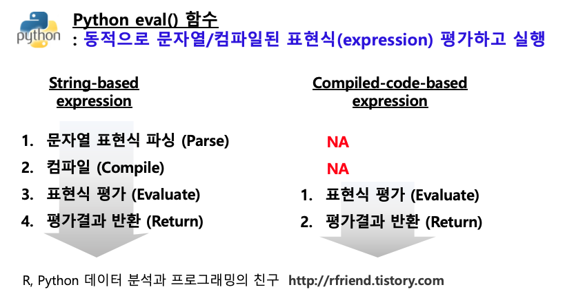
Python 의 내장함수(built-in function)인 eval() 함수는 임의의 문자열 기반(string-based) 또는 컴파일된 코드 기반 (compiled-code-based) 인풋의 표현식(expressions)을 평가(evaluate)해서 실행해줍니다. 

문자열 기반의 표현식을 eval() 함수가 처리하는 순서는 아래와 같습니다. 

  (1-a) 문자열 기반 표현식을 파싱한다. (Parse a string-based expression)

  (1-b) 문자열을 파싱한 결과를 바이트코드로 컴파일한다. (Compile it to bytecode)

  (1-c) 파이썬 표현식으로 평가한다. (Evaluate it as a Python expression) 

  (1-d) 평가한 결과를 하나의 값으로 반환한다. (Return the result of the evaluation)

아래 예시는 문자열 기반 표현식 (string-based expressions) 으로 수학 계산식(math expressions)을 인풋으로 해서 eval() 메소드를 사용해 동적으로 평가하여 실행한 것입니다. 

## You can use the built-in Python eval() 
## to dynamically evaluate expressions 
## from a string-based or compiled-code-based input.

##-- eval() for a string-based input
##-- Math expressions
eval("2 + 6")
# 8

eval("10**2")
# 100

eval("sum([1, 2, 3, 4, 5])")
# 15


import math
eval("math.pi * pow(5, 2)")
# 78.53981633974483

eval() 함수는 문자열 표현식에서 아래 예의 x 와 같은 글로벌 변수에 접근해서 표현식을 평가하고 실행할 수 있습니다.  

## eval() has access to global names like x
x = 10
eval("x * 5")
# 50

eval() 함수는 문자열의 블리언 표현식 (Boolean expressions)에 대해서도 평가하여 실행할 수 있습니다.

아래의 예에서는 순서대로 블리언 표현식 (Boolean expressions)의 

  (a) 비교 연산자 (value comparison operstors: <, >, <=, >=, ==, !=)),

  (b) 논리 연산자 (logical operators: and, or, not),

  (c) 소속 여부 확인 연산자 (membership test operators: in, not in),

  (d) 동일 여부 확인 연산자 (identity operators: is, is not)

을 사용한 문자열 기반 인풋을 eval() 메소드를 통해 평가하고 실행해 보았습니다. 

## -- eval() for Boolean expressions
x = 10

## (a) value comparison operators: <, >, <=, >=, ==, !=
eval("x > 5")
# True


## (b) logical operstors: and, or, not
eval("x > 5 and x < 9")
# False


## (c) membership test operators: in, not in
eval("x in {1, 5, 10}")
# True


## (d) identity operators: is, is not
eval("x is 10")
# True

그러면, 그냥 Python 표현식을 쓰면 되지, 왜 굳이 문자열 기반의 표현식을 eval() 함수에 인풋으로 넣어서 쓸까 궁금할 것입니다. 아래의 조건 표현식을 가지는 사용자 정의 함수를 예로 들자면, 사용자 정의함수 myfunc() 를 사용할 때처럼 동적으로 문자열 기반의 조건절 표현식을 바꾸어가면서 쓸 수 있어서 강력하고 편리합니다. 

## suppose you need to implement a conditional statement, 
## but you want to change the condition on the fly, dynamically. 
def myfunc(a, b, condition):
    if eval(condition):
        return a + b
    return a - b
    
    
myfunc(5, 10, "a > b")
# -5


myfunc(5, 10, "a <= b")
# 15


myfunc(5, 10, "a is b")
# -5

(2) eval() 함수의 잘못된 사용 예시 (SyntaxError) 

(2-1) 만약 eval() 함수의 인풋으로 표현식(expressions) 이 아니라, if, while 또는 for 와 같은 키워드를 사용해서 만든 코드 블락으로 이루어진 명령문(statement)을 사용한다면 "SyntaxError: invalid syntax" 에러가 발생합니다. 

## if you pass a compound statement to eval(), 
## then you'll get a SyntaxError. 
x = 10
eval("if x>5: print(x)")
# File "<string>", line 1
#     if x>5: print(x)
#     ^
# SyntaxError: invalid syntax

(2-2) eval() 함수에 할당 연산(assignment operations: =) 을 사용하면 "SyntaxError: invalid syntax" 에러가 발생합니다. 

## Assignment operations aren't allowed with eval(). 
eval("x = 10")
# File "<string>", line 1
#     x = 10
#       ^
# SyntaxError: invalid syntax

(2-3) Python 구문의 규칙을 위배하면 "SyntaxError: unexpedted EOF while parsing" 에러가 발생합니다. 

(아래 예에서는 "1 + 2 -" 에서 문자열 마지막에 - 부호가 잘못 들어갔음) 

## If an expression violates Python syntax, then SyntaxError
eval("1 + 2 -")
# File "<string>", line 1
#     1 + 2 -
#           ^
# SyntaxError: unexpected EOF while parsing

(3) compiled-code-based 인풋을 eval() 함수에 사용하기

eval() 함수의 인풋으로 위의 문자열 기반 객체 대신 compiled-code-based 객체를 사용할 수도 있습니다. compiled-code-based 객체를 eval() 함수의 인풋으로 사용하면 아래의 두 단계를 거칩니다. 

  (3-a) 컴파일된 코드를 평가한다. (Evaluate the compiled code)

  (3-b) 평가 결과를 반환한다. (Return the result of the evaluation)

위의 (1)번에서 문자열 기반의 표현식을 eval() 함수의 인풋으로 사용했을 때 대비 compiled-code 객체를 eval() 함수의 인풋으로 사용할 경우 파싱하고 컴파일 하는 단계가 없고, 바로 컴파일된 코드를 평가하고 반환하는 단계로 넘어가므로 똑같은 표현식을 여러번 평가해야 하는 경우에 속도 향상을 기대할 수 있습니다. 

Python의 eval() 함수에 compiled code 객체를 인풋으로 사용하려면, 

compiled_code_object = compile(source, filename, mode) 의 구문을 사용해서 컴파일 해주면 됩니다. 

 - source 에는 문자열 표현식(string-based expression)을 넣어줍니다. 

 - filename 에는 문자열 기반 표현식을 사용할 경우 "<string>" 을 써줍니다. 

 - mode 에는 컴파일된 코드를 eval() 함수로 처리하길 원할 경우 "eval" 을 써줍니다. 

##-- eval() for compiled-code-based input
compiled_code = compile("(2 + 3) * 10", "<string>", "eval")
eval(compiled_code)
# 50

[ Reference ]

* Real Python site: "Python eval(): Evaluate Expressions Dynamically
: https://realpython.com/python-eval-function/

이번 포스팅이 많은 도움이 되었기를 바랍니다 .

행복한 데이터 과학자 되세요! :-)

이번 포스팅에서는 유닉스 스타일로 Python의 파일 경로와 파일명 패턴 매칭을 통해 찾아주는 glob, fnmatch 모듈에 대해서 알아보겠습니다. 

(1) glob: 유닉스 스타일 경로명 패턴 확장 (Unix style pathname pattern expansion)

(2) fnmatch: 유닉스 스타일 파일명 패턴 매칭 (Unix style filename pattern matching)

(1) glob: 유닉스 스타일 경로명 패턴 확장 (Unix style pathname pattern expansion)

Python의 glob 모듈은 Unix shell에서 사용되는 규칙에 따라 지정된 패턴과 일치하는 모든 경로 이름을 찾아주며, 결과는 임의의 순서로 반환합니다. 

간단한 예를 들어서 설명해보겠습니다. 아래와 같은 파일경로의 계층으로 여러개의 파일이 있습니다. 

- data > glob 폴더내 'glob.ipynb' 파일, train 하위 폴더, test 하위 폴더

- data > glob > train 폴더 내 '1.txt', '2.txt', '1001.txt', '1002.txt', 'a.txt', 'b.txt', 'cat.jpeg'

- data > glob > test 폴더 내 '4.txt', '5.txt', 'd.txt', e.txt'

(1-1) glob.glob('./*'): 현재 폴더의 폴더와 파일 경로 가져오기

import glob

## 현재 폴더의 폴더와 파일 경로
glob.glob('./*')

# ['./test', './glob.ipynb', './train']

(1-2) glob.glob(./foldername/*'): 특정 폴더 내 모든 파일 경로 가져오기

## ''./train' 경로의 모든 파일 경로
glob.glob('./train/*')

# ['./train/cat.jpeg',
#  './train/b.txt',
#  './train/a.txt',
#  './train/2.txt',
#  './train/1002.txt',
#  './train/1.txt',
#  './train/1001.txt']

(1-3) glob: 특정 폴더 내 특정 파일이름으로 끝나는 모든 파일 경로 가져오기 

예 1) '.txt' 로 끝나는 파일 경로

## '.txt' 로 끝나는 파일 경로
glob.glob('./train/*.txt')

# ['./train/b.txt',
#  './train/a.txt',
#  './train/2.txt',
#  './train/1002.txt',
#  './train/1.txt',
#  './train/1001.txt']

예 2) '.jpeg' 로 끝나는 파일 경로 

## '.jpeg' 로 끝나는 파일 경로
glob.glob('./train/*.jpeg')

# ['./train/cat.jpeg']

(1-4) glob.glob([0-9]*): 0~9 숫자로 시작하는 파일 경로 가져오기

## 0~9 숫자로 시작하는 파일 경로
glob.glob('./train/[0-9]*')

# ['./train/2.txt', 
#  './train/1002.txt', 
#  './train/1.txt', 
#  './train/1001.txt']

(1-5) glob.glob('./**/*', recursive=True)
  : 현재 폴더에 있는 폴더와 파일, 하위 폴더 내 모든 파일 경로 재귀적으로 가져오기

## ''**/*' 와 recursive=True : 현재 폴더에 있는 폴더와 파일, 하위 폴더 내 경로 재귀적으로 가져오기 
glob.glob('./**/*', recursive=True)

# ['./test',
#  './glob.ipynb',
#  './train',
#  './test/5.txt',
#  './test/4.txt',
#  './test/e.txt',
#  './test/d.txt',
#  './train/cat.jpeg',
#  './train/b.txt',
#  './train/a.txt',
#  './train/2.txt',
#  './train/1002.txt',
#  './train/1.txt',
#  './train/1001.txt']

(1-6) glob.glob('./**/*/', recursive=True): 현재 폴더에 있는 폴더 경로만 가져오기

## 제일 마지막에 '/' 추가: 폴더만
glob.glob('./**/*/', recursive=True)

# ['./test/', './train/']

(1-7) 디렉토리(<DIR>)와 파일(<FILE>) 구분자 추가해서 프린트 하기

import glob
from os.path import isdir

for x in glob.glob('./**/*', recursive=True):
    if isdir(x):
        print('<DIR> ', x) # 디렉토리
    else:
        print('<FILE>', x) # 파일
        
# <DIR>  ./test
# <FILE> ./glob.ipynb
# <DIR>  ./train
# <FILE> ./test/5.txt
# <FILE> ./test/4.txt
# <FILE> ./test/e.txt
# <FILE> ./test/d.txt
# <FILE> ./train/cat.jpeg
# <FILE> ./train/b.txt
# <FILE> ./train/a.txt
# <FILE> ./train/2.txt
# <FILE> ./train/1002.txt
# <FILE> ./train/1.txt
# <FILE> ./train/1001.txt

(1-8) 재귀하면서(recursive=True) 모든 폴더 내 파일 이름만 리스트로 가져오기

## 모든 폴더 내 파일 이름만 가져오기
import os

fnames = [
    os.path.basename(x) # 파일 이름
    for x in glob.glob('./**/*', recursive=True) # 재귀하면서 폴더&파일경로
    if not isdir(x) # 폴더 제외
]

print(fnames)

# ['glob.ipynb', 
#  '5.txt', 
#  '4.txt', 
#  'e.txt', 
#  'd.txt', 
#  'cat.jpeg', 
#  'b.txt', 
#  'a.txt', 
#  '2.txt', 
#  '1002.txt', 
#  '1.txt', 
#  '1001.txt']

(1-9) 재귀 대신 매뉴얼하게 모든 폴더를 지정해주어서 파일 이름만 리스트로 가져오기

 : 위의 (1-8) 재귀문과 결과 동일. 하위 폴더 개수가 많을 수록 (1-9) 수작업 코드 복잡해지고, 자동화에 제약 있음. 

## 파일 이름만 가져오기 : os.listdir() 이용해서
## 재귀 대신 매뉴얼하게 모든 폴더를 써줘야 함
import os

os.listdir('./') + os.listdir('./train/') + os.listdir('./test/')

# ['.DS_Store',
#  'test',
#  'glob.ipynb',
#  'train',
#  '.ipynb_checkpoints',
#  'cat.jpeg',
#  '.DS_Store',
#  'b.txt',
#  'a.txt',
#  '2.txt',
#  '1002.txt',
#  '1.txt',
#  '1001.txt',
#  '.DS_Store',
#  '5.txt',
#  '4.txt',
#  'e.txt',
#  'd.txt']

(1-10) 반복자(iterator) 반환하여 for loop 순환문에 사용하기

# glob.iglob(): 반복자(iterator) 반환
path_iterator = glob.iglob('./train/**.txt')

for path in path_iterator:
    print(path)
    
# ./train/b.txt
# ./train/a.txt
# ./train/2.txt
# ./train/1002.txt
# ./train/1.txt
# ./train/1001.txt

(2) fnmatch: 유닉스 스타일 파일명 패턴 매칭 (Unix style filename pattern matching)

fnmatch.fnmatch(filename, pattern) 메소드는 faiename 문자열이 pattern 문자열과 일치하는지를 검사하여, True나 False 를 반환합니다. 패턴 매칭하는 구문은 아래와 같습니다. 

    [seq] : seq 의 모든 문자와 일치합니다. 

    * : 모든 것과 일치합니다. 

(2-1) 특정 폴더 내 숫자로 시작('[0-9]*')하는 모든 파일 이름 가져오기

## filename 문자열이 pattern 문자열과 일치하는지를 검사하여, True 나 False를 반환합니다.
import fnmatch
import os

for file in os.listdir('./train'):
    # [seq]  seq의 모든 문자와 일치합니다.
    # *      모든 것과 일치합니다
    if fnmatch.fnmatch(file, '[0-9]*'):
        print(file)
        
# 2.txt
# 1002.txt
# 1.txt
# 1001.txt

(2-2) 특정 폴더 내 문자로 시작([!0-9]*')하는 모든 파일 이름 가져오기

for file in os.listdir('./train'):
    # [!seq] seq에 없는 모든 문자와 일치합니다
    if fnmatch.fnmatch(file, '[!0-9]*'):
        print(file)
        
# cat.jpeg
# b.txt
# a.txt

(2-3) 특정 폴더 내 특정 문자열로 끝나는 파일 이름 가져오기

for file in os.listdir('./train'):
    # *      모든 것과 일치합니다
    if fnmatch.fnmatch(file, '*.jpeg'):
        print(file)
        
# cat.jpeg

(2-4) 특정 폴더 내 모든 단일 문자('?')와 일치하는 파일 이름 가져오기

for file in os.listdir('./train'):
    # ?      모든 단일 문자와 일치합니다
    if fnmatch.fnmatch(file, '?.txt'):
        print(file)
        
# b.txt
# a.txt
# 2.txt
# 1.txt

(2-5) 특정 폴더 내 모든 파일 이름 가져오기

for file in os.listdir('./train'):
    # *      모든 것과 일치합니다
    if fnmatch.fnmatch(file, '*.txt'):
        print(file)
        
# b.txt
# a.txt
# 2.txt
# 1002.txt
# 1.txt
# 1001.txt

[Reference]

- glob module: https://docs.python.org/3/library/glob.html

- fnmatch module: https://docs.python.org/3/library/fnmatch.html#module-fnmatch

이번 포스팅이 많은 도움이 되었기를 바랍니다. 

행복한 데이터 과학자 되세요! :-)

이번 포스팅에서는 Python을 사용해서 파워포인트와 PDF 파일에서 텍스트를 추출하는 방법을 소개하겠습니다. 

(1) 파워포인트 파일에서 텍스트 추출하기 (Extracting text from a PowerPoint file)

(2) PDF 파일에서 텍스트 추출하기 (Extracting text from a PDF file)

예제로 사용할 파워포인트와 PDF 파일 첨부합니다. 

* 예제 파워포인트 파일: "서울관광명소.pptx"

* 예제 PDF 파일: "서울관광명소.pdf"

예제로 사용하는 "서울관광명소.pptx" 파일은 아래와 같이 텍스트로 구성되어 있습니다. 

(1) 파워포인트 파일에서 텍스트 추출하기 (Extracting text from a PowerPoint file)

Python으로 파워포인트에 파일에서 텍스트를 추출하기 위해서 먼저 테미널에서 "python-pptx" 모듈을 설치합니다. 

% python -m pip install python-pptx

파워포인트 파일이 저장되어 있는 경로와 파일 이름을 설정해주고, python-pptx 모듈을 사용해서 파워포인트 파일로 부터 텍스트를 추출해보겠습니다. 

이때 가독성을 높이기 위해서 각 슬라이드의 제목(title)을 Key 로 하고, 각 슬라이드의 본문 내용을 Value 로 하는 사전형(Dictionary) 형태로 추출한 텍스트를 저장해보겠습니다. 

## setting directory and file names
base_dir = "/Users/lhongdon/Documents/" # set with yours
ppt_nm = "서울관광명소.pptx"
pdf_nm = "서울관광명소.pdf"

ppt_path = base_dir + ppt_nm
pdf_path = base_dir + pdf_nm

print(ppt_path)
print(pdf_path)
# /Users/lhongdon/Documents/서울관광명소.pptx
# /Users/lhongdon/Documents/서울관광명소.pdf


## (1) extracting text from a PowerPoint file
from pptx import Presentation

prs = Presentation(ppt_path)

# text_runs will be populated with a list of strings,
# one for each text run in presentation
text_runs = {}

for slide in prs.slides:
    text_run = []
    for shape in slide.shapes:
        if not shape.has_text_frame:
            continue
        for paragraph in shape.text_frame.paragraphs:
            for run in paragraph.runs:
                text_run.append(run.text)

    text_runs[text_run[0]] = text_run[1:]
    
    
    
 print(text_runs)

# {'서울의 관광 명소': ['서울의 랜드마크', '서울의 고궁', '서울의 미술관과 박물관'],
#  '서울의 랜드마크': ['명동성당', '익선동 한옥거리', '광화문광장 야경', '롯데월드타워', '서울광장', '청와대'],
#  '서울의 고궁': ['경복궁', '창덕궁', '창경궁', '덕수궁', '서울 한양도성', '홍인지문', '숭례문'],
#  '서울의 미술관과 박물관': ['호림박물관', '갤러리 학고재', '별마당 도서관', '전쟁기념관', '국립중앙박물관']}

(2) PDF 파일에서 텍스트 추출하기 (Extracting text from a PDF file)

Python의 PyPDF2 모듈을 이용해서 PDF 파일로 부터 텍스트를 추출하기 위해, 먼저 터미널에서 "PyPDF2" 모듈을 설치합니다.  

% python -m pip install PyPDF2

다음으로, PdfReader() 메소드를 사용해서 각 PDF 페이지로부터 텍스트를 추출해서 text_all 이라는 리스트에 차곡차곡 합쳐보도록 하겠습니다. 

from PyPDF2 import PdfReader

## initiate PdfReader
reader = PdfReader(pdf_path)

print(len(reader.pages))
# 4


## extract text from a pdf file
text_all = []

for page in reader.pages:
    text = page.extract_text()
    text_all.append(text)
    


print(text_all)
# ['서울의관광명소1.서울의랜드마크2.서울의고궁3.서울의미술관과박물관',
#  '서울의랜드마크•명동성당•익선동한옥거리•광화문광장야경•롯데월드타워•서울광장•청와대',
#  '서울의고궁•경복궁•창덕궁•창경궁•덕수궁•서울한양도성•홍인지문•숭례문',
#  '서울의미술관과박물관•호림박물관•갤러리학고재•별마당도서관•전쟁기념관•국립중앙박물관']

이번 포스팅이 많은 도움이 되었기를 바랍니다. 

행복한 데이터 과학자 되세요!  :-)

이번 포스팅에서는 인덱스 반복자(iterator) enumerate() 와 numpy 의 다차원 배열에 대한 인덱스 반복자 (multidimensional index iterator) np.ndenumerate(arr) 메소드에 대해서 소개하겠습니다. 

(1) 인덱스 반복자 (index iterator): enumerate()

(2) 다차원 배열 (multidimensional index iterator): numpy.ndenumerate(arr)

반복(iteration) 이란 일련의 작업 명령문을 반복해서 실행(repeated execution)하는 것을 말합니다. Python은 이러한 반복 작업을 더 쉽게 수행할 수 있도록 하는 여러 언어 기능이 있습니다.

반복자(iterator)는 반복할 수 있는 값의 수를 계산하는 객체입니다. Python의 데이터 유형 중에서 리스트(Lists), 튜플(Tuples), 사전형(Dictionaries), 문자열(Strings), 집합(Sets) 이 모두 반복 가능한 객체들로서, 반복자(iterator)를 가져올 수 있습니다. 

(1) 인덱스 반복자 (index iterator): enumerate()

Python에서는 for loop 순환문이 종종 반복가능한 객체에 순환 반복문으로 사용이 됩니다. for loop 문을 사용하면 인덱스 또는 순환하는 횟수는 반환하지 않고, 오로지 반복가능한 객체의 원소만을 반환하게 됩니다.

아래 예에서는 리스트(list)에 for loop 문을 사용해서 리스트 안의 원소를 하나씩 순서대로 반복해서 프린트하는 코드입니다. (이때 인덱스 정보는 없음)  

## (1) without index iterator
x_list = ['a', 'b', 'c', 'd']

for x in x_list:
    print('item:', x)
    
# item: a
# item: b
# item: c
# item: d

만약 for loop 순환문을 반복가능한 객체에 사용하면서 enumerate() 메소드를 사용하면 쉽고 편리하게 인덱스 정보 (index information)을 같이 반환할 수 있습니다.

아래 예에서는 enumerate(x_list) 를 for loop 순환문과 같이 사용해서 '인덱스 정보(index information) + 리스트 내 원소 정보'를 순환하면서 반복적으로 프린트해보았습니다. 

## (2) enumerate()
## : iteration with access to the index information
x_list = ['a', 'b', 'c', 'd']
print(x_list)

print('----' * 5)

for i, x in enumerate(x_list):
    print('index:', i, '  item:', x)
    

# ['a', 'b', 'c', 'd']
# --------------------
# index: 0   item: a
# index: 1   item: b
# index: 2   item: c
# index: 3   item: d

(2) 다차원 배열 (multidimensional index iterator): numpy.ndenumerate(arr)

numpy 의 다차원 배열 (multidimensional array)에 대해서 위의 (1) enumerate() 메소드가 했던 것처럼 반복 가능한 객체에 대해 인덱스 정보를 가져오고 싶다면 numpy.ndenumerate(arr) 메소드를 사용하면 됩니다. 

아래 예에서는 3차원 배열(3 dimensional array) 에 대해서 for loop 순환문과 np.ndenumerate(arr) 메소드를 같이 사용해서 3차원 배열의 인덱스 정보 (index information of 3 dimensional array) 와 원소를 순환하면서 반복적으로 프린트해보았습니다. 

## numpy.ndenumerate(arr)
## : multidimensional index iterator

import numpy as np

y_3d_arr = np.array([[[1, 2], [3, 4]], [[5, 6], [7, 8]]])
print(y_3d_arr)

print('------' * 5)

for i, y in np.ndenumerate(y_3d_arr):
    print('index:', i, '  item:', y)
    
# [[[1 2]
#   [3 4]]

#  [[5 6]
#   [7 8]]]
# ------------------------------
# index: (0, 0, 0)   item: 1
# index: (0, 0, 1)   item: 2
# index: (0, 1, 0)   item: 3
# index: (0, 1, 1)   item: 4
# index: (1, 0, 0)   item: 5
# index: (1, 0, 1)   item: 6
# index: (1, 1, 0)   item: 7
# index: (1, 1, 1)   item: 8

반복 가능한 객체로 리스트(Lists), 튜플(Tuples), 사전형(Dictionaries), 문자열(Strings), 집합(Sets) 등이 있다고 했는데요, 아래 예에서는 다차원 리스트에 대해서 for loop 순환문과 np.ndenumerate() 메소드를 같이 사용해서 인덱스 정보와 리스트 내 원소를 순환하면서 반복적으로 인쇄를 해보았습니다. 

## iterable objects: Lists, Tuples, Dictionaries, Strings, Sets

x_2d_list = [['a', 'b'], ['c', 'd']]
print(x_2d_list)

print('-----' * 5)

for i, x in np.ndenumerate(x_2d_list):
    print('index:', i, '  item:', x)
    
# [['a', 'b'], ['c', 'd']]
# -------------------------
# index: (0, 0)   item: a
# index: (0, 1)   item: b
# index: (1, 0)   item: c
# index: (1, 1)   item: d

이번 포스팅이 많은 도움이 되었기를 바랍니다 .

행복한 데이터 과학자 되세요. :-)

지난번 포스팅에서는 분류 모델(classification model)의 성능을 평가할 수 있는 지표 (evaluation metrics)에 대해서 소개하였습니다. (https://rfriend.tistory.com/771)

이번 포스팅에서는 Python을 사용하여 예제 데이터에 대해 분류 모델의 성능 평가를 해보겠습니다. 

(1) 예제로 사용할 Breast Cancer 데이터셋을 로딩하고, Data와 Target으로 구분

(2) Training set, Test set 분할

(3) Logistic Regression 모델 적합 (Training)

(4) 예측 (Prediction)

(5) 혼돈 매트릭스 (Confusion Matrix)

(6) 분류 모델 성능 지표: Accuracy, Precision, Recall rate, Specificity, F-1 score

(7) ROC 곡선, AUC 점수

(1) 예제로 사용할 Breast Cancer 데이터셋을 로딩하고, Data와 Target으로 구분 

target의 '0' 이 'malignant (악성 종양)' 이고, '1'은 'benign' 으로서 정상을 의미합니다. 우리는 'malignant (악성 종양)' 을 분류하는 모델에 관심이 있으므로 target '0' 이 'Positive Label' 이 되겠습니다. 

import numpy as np

## load a Iris dataset
from sklearn.datasets import load_breast_cancer

bc = load_breast_cancer()

## target names
bc.target_names
#array(['malignant', 'benign'], dtype='<U9')

## [0: 'malignant'(악성), 1: 'benign']
np.unique(bc['target'], return_counts=True) 
#(array([0, 1]), array([212, 357]))


## getting data, target
bc_data = bc['data']
bc_target = bc['target']

bc_data.shape
#(569, 30)

bc_target[:20]
#array([0, 0, 0, 0, 0, 0, 0, 0, 0, 0, 0, 0, 0, 0, 0, 0, 0, 0, 0, 1])

(2) Training set, Test set 분할

Training set 0.5, Test set 0.5 의 비율로 무작위 추출하여 분할하였습니다. 

## splits training and test set
from sklearn.model_selection import train_test_split

X_train, X_test, y_train, y_test = train_test_split(
    bc_data, 
    bc_target, 
    test_size=0.5,  
    random_state=1004
)

(3) Logistic Regression 모델 적합 (Training)

Traning set을 사용해서 로지스틱 회귀모형을 적합하였습니다.

## training a Logistic Regression model with training set
from sklearn.linear_model import LogisticRegression

clf = LogisticRegression(
    solver='liblinear', 
    random_state=1004).fit(X_train, y_train)

(4) 예측 (Prediction)

Test set에 대해서 예측을 하고 모델 성능 평가를 해보겠습니다. 

predict() 메소드는 범주를 예측하여 반환하고, predict_praba() 메소드는 확률(probability)을 반환합니다. 

## prediction for test set
y_pred = clf.predict(X_test) # class
y_pred_proba = clf.predict_proba(X_test) # probability

실제 범주의 값과 예측한 범주의 값, 그리고 target '0'(malignant, 악성 종양) 일 확률을 DataFrame으로 묶어보았습니다. 

# All in a DataFrame
pred_df = pd.DataFrame({
    'actual_class': y_test, 
    'predicted_class': y_pred, 
    'probabilty_class_0': y_pred_proba[:,0] # malignant (악성)
})

pred_df.head(10)
#    actual_class  predicted_class  probabilty_class_0
# 0             1                1            0.002951
# 1             0                0            0.993887
# 2             0                1            0.108006
# 3             1                1            0.041777
# 4             0                0            1.000000
# 5             0                0            1.000000
# 6             0                0            0.999633
# 7             1                1            0.026465
# 8             0                0            0.997405
# 9             1                1            0.002372

이제 여기서부터 분류 모델의 성능 평가를 시작합니다. 

(5) 혼돈 매트릭스 (Confusion Matrix)

혼돈 매트릭스의 Y축은 Actual 의 malignant (0), benign(1) 이며, X 축은 Predicted 의 malignant (0), benign(1) 입니다. 

## model evaluation
# Confusion matrix
from sklearn.metrics import confusion_matrix

confusion_matrix(y_test, y_pred, 
                 labels=[0, 1]) # 'malignant'(0), 'benign'(1)

#                   predicted
#                   malignant  benign
# actual malignant [[102,       16],
#        benign    [  3,       164]])

(6) 분류 모델 성능 지표: Accuracy, Precision, Recall rate, Specificity, F-1 score

from sklearn.metrics import accuracy_score
from sklearn.metrics import precision_recall_fscore_support

## performance metrics
accuracy = accuracy_score(y_test, y_pred)

precision, recall, fscore, support = \
    precision_recall_fscore_support(y_test, y_pred)

print('Accuracy   : %.3f' %accuracy) # (102+164)/(102+16+3+164)
print('Precision  : %.3f' %precision[0]) # 102/(102+3)
print('Recall     : %.3f' %recall[0]) # 102/(102+16)
print('Specificyty: %.3f' %recall[1]) # 164/(3+164)
print('F1-Score   : %.3f' %fscore[0]) # 2/(1/precision + 1/recall) = 2/(1/0.971+1/0.864)

# Accuracy   : 0.933
# Precision  : 0.971
# Recall     : 0.864
# Specificyty: 0.982
# F1-Score   : 0.915

sklearn의 classification_report() 메소드를 활용해서 한꺼번에 쉽게 위의 분류 모델 성능평가 지표를 계산하고 출력할 수 있습니다. 참고로, 'macro avg' 는 가중치가 없는 평균이며, 'weighted avg'는 support (관측치 개수) 로 가중치를 부여한 평균입니다. 

from sklearn.metrics import classification_report

target_names = ['malignant(0)', 'benign(1)']
print(classification_report(y_test, y_pred, 
                            target_names=target_names))

#               precision    recall  f1-score   support

# malignant(0)       0.97      0.86      0.91       118
#    benign(1)       0.91      0.98      0.95       167

#     accuracy                           0.93       285
#    macro avg       0.94      0.92      0.93       285
# weighted avg       0.94      0.93      0.93       285

(7) ROC 곡선, AUC 점수

ROC 곡선과 AUC 점수는 예측 확률을 이용합니다.

ROC 곡선은 모든 의사결정 기준선 (decision threshold)에 대하여 혼돈 매트릭스를 만들고, X축에는 False Positive Rate(=1-specificity), Y축에는 True Positive Rate (=recall, sensitivity) 의 값을 선그래프로 그린 것이며, 좌측 상단으로 그래프가 붙을 수록 더 잘 적합된 모델이라고 평가합니다. AUC 점수는 ROC 곡선의 아랫부분의 면적을 적분한 값입니다. 

## ROC Curve, AUC
import sklearn.metrics as metrics

fpr, tpr, threshold = metrics.roc_curve(
    y_test, 
    y_pred_proba[:, 0], 
    pos_label=0) # positive label

AUC = metrics.auc(fpr, tpr)

# plotting ROC Curve
import matplotlib.pyplot as plt

plt.figure(figsize = (8, 8))
plt.plot(fpr, tpr, 'b', label = 'AUC = %0.3f' % AUC)
plt.title(('ROC Curve of Logistic Regression'), fontsize=18)
plt.legend(loc = 'lower right')

plt.plot([0, 1], [0, 1],'r--') # random guess
plt.xlim([0, 1])
plt.ylim([0, 1])
plt.ylabel('True Positive Rate', 
                fontsize=14)
plt.xlabel('False Positive Rate', 
                fontsize=14)

plt.show()

[ Reference ] 

1) Breast Cancer Dataset
: https://scikit-learn.org/stable/modules/generated/sklearn.datasets.load_breast_cancer.html

2) Scikit-Learn Logistic Regression
: https://scikit-learn.org/stable/modules/generated/sklearn.linear_model.LogisticRegression.html

3) 분류 모델의 성과 평가 지표 : https://rfriend.tistory.com/771

이번 포스팅이 많은 도움이 되었기를 바랍니다. 

행복한 데이터 과학자 되세요!  :-)

이번 포스팅에서는 여러개의 칼럼을 가지는 pandas DataFrame에서 특정 데이터 유형의 칼럼을 선택하거나 배제하는 방법을 소개하겠습니다. 

(1) pandas DataFrame 의 칼럼별 데이터 유형 확인: df.dtypes

(2) pandas DataFrame 에서 특정 데이터 유형의 칼럼을 선택하기: df.select_dtypes(include)

(3) pandas DataFrame 에서 특정 데이터 유형의 칼럼을 제외하기: df.select_dtypes(exclude)

먼저, 예제로 사용할 pandas DataFrame을 만들어보겠습니다. 데이터 유형으로는 int64, object, boolean, folat64, datetime64 의 5개 서로 다른 유형을 포함하도록 하였습니다. 

import pandas as pd

## sample pandas DataFrame
df = pd.DataFrame({
    'x1': [1, 2, 3], # int64
    'x2': ['a', 'b', 'c'], # object
    'x3': [True, False, False], # boolean
    'x4': [1.0, 2.0, 3.0], # float64
    'x5': [pd.Timestamp('20230101'), pd.Timestamp('20230102'), pd.Timestamp('20230103')] # datetime64
})


print(df)
#    x1 x2     x3   x4         x5
# 0   1  a   True  1.0 2023-01-01
# 1   2  b  False  2.0 2023-01-02
# 2   3  c  False  3.0 2023-01-03
# 3   4  d   True  4.0 2023-01-04

(1) pandas DataFrame 의 칼럼별 데이터 유형 확인: df.dtypes

## (1) pd.DataFrame.dtypes: data type of each column.

df.dtypes
# x1             int64
# x2            object
# x3              bool
# x4           float64
# x5    datetime64[ns]
# dtype: object

(2) pandas DataFrame 에서 특정 데이터 유형의 칼럼을 선택하기 (include)

pd.DataFrame.select_dtypes(include=None) 메소드를 사용하여 원하는 데이터 유형을 include = 'data type' 옵션에 넣어주면 됩니다. 아래 예시에서는 차례대로 include='int64', 'object', 'bool', float64', 'datetime64' 별로  칼럼을 선택해보았습니다. 

## (2) DataFrame.select_dtypes(include=None, exclude=None)
## Return a subset of the DataFrame’s columns based on the column dtypes.

## including the dtypes in include.
df.select_dtypes(include='int64') # int
# x1
# 0	1
# 1	2
# 2	3
# 3	4


df.select_dtypes(include='object')
# x2
# 0	a
# 1	b
# 2	c
# 3	d


df.select_dtypes(include='bool')
# x3
# 0	True
# 1	False
# 2	False
# 3	True


df.select_dtypes(include='float64') # float
# x4
# 0	1.0
# 1	2.0
# 2	3.0
# 3	4.0


df.select_dtypes(include='datetime64') # datetime
# x5
# 0	2023-01-01
# 1	2023-01-02
# 2	2023-01-03
# 3	2023-01-04

한꺼번에 여러개의 데이터 유형의 칼럼을 선택하고자 할 때는 df.select_dtypes(include=[dtype1, dtype2, ...]) 처럼 include 옵션에 여러개의 데이터 유형을 리스트로 넣어주면 됩니다. 아래 예시에서는 ['int64', 'float64'] 의 두 개의 숫자형 칼럼을 선택해 보았습니다. 

숫자형 (numeric data type) 의 칼럼을 선택하는 또 다른 방법은 df.select_dtypes(include='number') 를 해도 됩니다. 

## (a) include=[dtype, dtype, ...]
df.select_dtypes(include=['int64', 'float64']) # 여러개의 data type

# x1	x4
# 0	1	1.0
# 1	2	2.0
# 2	3	3.0
# 3	4	4.0



## (b) To select all numeric types, use np.number or 'number'
df.select_dtypes(include='number') # int, float

# x1	x4
# 0	1	1.0
# 1	2	2.0
# 2	3	3.0
# 3	4	4.0

숫자형('int64', 'float64') 의 칼럼 이름을 리스트로 반환하려면 columns 로 칼럼 이름을 가져와서 list() 로 묶어주면 됩니다. 

## column names of numeric types
list(df.select_dtypes(include='number').columns)

# ['x1', 'x4']

(3) pandas DataFrame 에서 특정 데이터 유형의 칼럼을 제외하기 (exclude)

위의 (2)번이 특정 데이터 유형을 포함(include)하는 칼럼을 선택하는 것이었다면, 이번에는 특정 데이터 유형을 제외(exclude) 한 나머지 칼럼을 선택하는 방법입니다. 아래 예시에서는 'int64' 데이터 유형을 제외(exclude='int64')한 나머지 칼럼을 반환하였습니다. 

## excluding the dtypes in exclude.
df.select_dtypes(exclude='int64')

# x2	x3	x4	x5
# 0	a	True	1.0	2023-01-01
# 1	b	False	2.0	2023-01-02
# 2	c	False	3.0	2023-01-03
# 3	d	True	4.0	2023-01-04

[Reference]

pandas.DataFrame.select_dtypes(include=None, exclude=None)
: https://pandas.pydata.org/docs/reference/api/pandas.DataFrame.select_dtypes.html

이번 포스팅이 많은 도움이 되었기를 바랍니다. 

행복한 데이터 과학자 되세요!  :-)

Python 리스트 자료형의 메소드와 내장함수에 대해서는 https://rfriend.tistory.com/330 를 참고하세요. 

이번 포스팅에서는 리스트(List) 자료형에 대한 유용한 활용 팁 네가지를 소개하려고 합니다. 

(1) 리스트의 문자형 원소를 숫자형 원소로 바꾸기 (혹은 그 반대)

(2) 리스트의 원소를 사전형의 Key:Value 기준으로 매핑하여 변환하기

(3) 리스트에서 또 다른 리스트의 겹치는 원소를 빼기

(4) 리스트 원소 정렬하기 (내림차순, 오름차순)

(1) 리스트의 문자형 원소를 숫자형 원소로 바꾸기 (혹은 그 반대)

list(map(data type, list)) 으로 리스트 내 원소의 데이터 유형을 변환할 수 있습니다. 아래는 순서대로 리스트 내 문자형 원소를 숫자형으로 변환, 숫자형 원소를 문자형 원소로 변환한 예입니다. 

## convert a list with string-type elements into a list with numeric-type elements
list(map(int, ['1', '2', '3']))  # 문자형 원소
# [1, 2, 3] # --> 숫자형으로 변환됨


## convert a list with numeric-type elements into a list with string-type elements
list(map(str, [1, 2, 3]))  # 숫자형 원소
# ['1', '2', '3'] # --> 문자형으로 변환됨

(2) 리스트의 원소를 사전형의 Key:Value 기준으로 매핑하여 변환하기

리스트 내 원소를 다른 값으로 변환할 때 사전형(Dictionary)의 Key:Value 매핑을 이용하면 편리합니다. List Comprehension 을 이용해서 리스트 원소별로 for loop 을 돌면서 Dictionary 의 Dict[Key] 로 Value에 접근해서 키별로 값을 매핑해서 변환된 값으로 새로운 리스트를 만들어줍니다. 

## a List
my_list = ['c', 'a', 'd', 'b']


## a Dictionary, which will be used for mapping, converting
my_dict = {
    'a': 1, 
    'b': 2, 
    'c': 3, 
    'd': 4
}

## accessing the value in a Dictionary using the key
my_dict['a']
# 1


## converting elements in a list using a Dictionary (Key: Value)
[my_dict[k] for k in my_list]
# [3, 1, 4, 2]

(3) 리스트에서 또 다른 리스트의 겹치는 원소를 빼기

리스트와 리스트 간 중복되는 원소 값 빼기는 TypeError: unsupported operand type(s) for -: 'list' and 'list' 에러를 반환합니다. 

## sample lists
a = [1, 2, 3, 4, 5]
b = [4, 5, 6, 7, 8]


## TypeError: unsupported operand type(s) for -: 'list' and 'list'
a - b
# ---------------------------------------------------------------------------
# TypeError                                 Traceback (most recent call last)
# <ipython-input-36-4dfa3698e4b8> in <module>
# ----> 1 a- b

# TypeError: unsupported operand type(s) for -: 'list' and 'list'

리스트 간 겹치는 값을 제거하려면 먼저 리스트를 Set 으로 변환을 해주고, 두 개의 Sets 간에 빼기를 해준 다음에, 집합 간 빼기 가 된 결과를 다시 list() 를 사용해서 리스트로 최종 변환해주면 됩니다. 

## substraction between lists using set
list(set(a) - set(b))
# [1, 2, 3]


list(set(b) - set(a))
# [8, 6, 7]

(4) 리스트 원소 정렬하기 (내림차순, 오름차순)

list.sort() 메소드를 사용해서 리스트 원소 (숫자형) 를 오름차순으로 정렬할 수 있습니다. 

내림차순 정렬을 하려면 list.sort(reverse=True) 처럼 옵션을 추가해주면 됩니다. 

## 리스트 원소 정렬
c = [8, 6, 7]
c.sort()
c
# [6, 7, 8]



## 리스트 원소 역순으로 정렬
c.sort(reverse=True)
c
# [8, 7, 6]

이번 포스팅이 많은 도움이 되었기를 바랍니다. 

행복한 데이터 과학자 되세요!  :-)

이번 포스팅에서는 Python의 Dictionary로 Key: Value 매핑하여 문자열을 변경해주는 replace() 함수를 사용하여 SQL query 코드의 여러개의 문자열을 변경하는 방법을 소개하겠습니다. 

코드가 길고 동일한 특정 변수나 테이블 이름이 여러번 나오는 경우, 수작업으로 일일이 하나씩 찾아가면서 변수나 테이블 이름을 변경하다보면 사람의 실수(human error)가 발생할 위험이 큽니다.  이럴 때 Dictionary에 (변경 전 : 변경 후) 매핑을 관리하고 컴퓨터에게 코드 변경을 시킬 수 있다면 사람의 실수를 예방하는데 도움이 될 것입니다. 

먼저, 예제로 사용할 SQL query와 Key(Before, 변경 전): Value(After, 변경 후) 를 매핑한 Dictionary 를 만들어보겠습니다. 

## key(Before): value(After) mapping dictionary
map_dict = {
    'X1': '"변수1"', # Key(Before): Value(After)
    'X2': '"변수2"', 
    'X3': '"변수3"',
    'MYTABLE': 'TEST_TABLE'
}


sql_query = "select \nx1, x2, x3 \nfrom mytable \nwhere x2 > 10 \nlimit 10;"

print(sql_query)
# select 
# x1, x2, x3 
# from mytable 
# where x2 > 10 
# limit 10;

아래에는 여러개의 줄(lines)을 가지는 문자열을 하나의 줄(line)로 나누어주는 splitlines() 메소드와, Dictionary의 Key, Value를 쌍으로 반환해주는 items() 메소드를 소개하였습니다. 

## splitlines()
for l in sql_query.splitlines():
    print(l)

# select 
# x1, x2, x3 
# from mytable 
# where x2 > 10 
# limit 10;



## replace(a, b) method convert a string 'a' with 'b'
s = 'Hello Python World.'
s.replace('Hello', 'Hi')

# 'Hi Python World.'



# dictionary.items() ==> returns key, value
for k, v in map_dict.items():
    print(k, ':', v)

# X1 : "변수1"
# X2 : "변수2"
# X3 : "변수3"
# MYTABLE : TEST_TABLE

위에서 기본적인 splitlines(), replace(), items() 메소드에 대한 사용법을 알았으니, 이제 이를 엮어서 코드에 있는 여러개의 특정 변수나 테이블 이름을 Dictionary(변경 전 이름 Key: 변경 후 이름 Value 매핑) 에서 가져와서 replace() 메소드로 변경해주는 사용자 정의함수를 만들어보겠습니다. 

## User Defined Function for converting codes 
## using replace() function and dictionary(Before: After mapping)
def code_converter(codes_old, map_dict):
    # blank string to save the converted codes
    codes_converted = ''
    
    # converting codes using replace() function and dictionary(Before: After mapping)
    for code in codes_old.splitlines():
        for before, after in map_dict.items():
            code = code.upper().replace(before, after)
            
        codes_converted = codes_converted + code + '\n'
        
    return codes_converted
    

## executing the UDF above
sql_query_new = code_converter(sql_query, map_dict)


print(sql_query_new)
# SELECT 
# "변수1", "변수2", "변수3" 
# FROM TEST_TABLE 
# WHERE "변수2" > 10 
# LIMIT 10;

이번 포스팅이 많은 도움이 되었기를 바랍니다. 

행복한 데이터 과학자 되세요!  :-)

지난번 포스팅에서는 독립된 2개 표본의 평균 차이를 검정하는 t-test 에 대해서 알아보았습니다. 
이번 포스팅에서는 Python을 이용한 짝을 이룬 표본의 평균 차이를 검정하는 paired t-test 에 대해서 소개하겠습니다. 
(R을 이용한 짝을 이룬 표본에 대한 평균 차이 검정은 https://rfriend.tistory.com/128 를 참고하세요)

짝을 이룬 t-test(paired t-test)는 짝을 이룬 측정치(paired measurements)의 평균 차이가 있는지 없는지를 검정하는 방법입니다. 데이터 값이 짝을 이루어서 측정되었다는 것에 대해 예를 들어보면, 사람들의 그룹에 대해 신약 효과를 알아보기 위해 (즉, 신약 투약 전과 후의 평균의 차이가 있는지) 신약 투약 전과 후(before-and-after)를 측정한 데이터를 생각해 볼 수 있습니다.  

[ One sample t-test vs. Independent samples t-test vs. Paired samples t-test ]

짝을 이룬 t-test(paired t-test)는 종속 표본 t-test (the dependent samples t-test), 짝을 이룬 차이 t-test (the paired-difference t-test), 매칭된 짝 t-test (the matched pairs t-test), 반복측정 표본 t-test (the repeated-sample t-teset) 등의 이름으로도 알려져있습니다. 동일한 객체에 대해서 전과 후로 나누어서 반복 측정을 합니다.  

아래의 도표에는 짝을 이룬 두 표본의 대응 비교 데이터셋에 대한 모습입니다. (Xi, Yi) 가 동일한 대상에 대해서 before-after 로 반복 측정되어서, 각 동일 객체의 전-후의 차이 (즉, Di = Xi - Yi) 에 대해서 검정을 진행하게 됩니다. 

[ 가정사항 (Assumptions) ]

(1) 측정 대상이 독립적(independent)이어야 합니다. 하나의 객체에 대한 측정은 어떤 다른 객체의 측정에 영향을 끼치지 않아야 합니다.  
(2) 각 짝을 이룬 측정치는 동일한 객체로 부터 얻어야 합니다. 예를 들면, 신약의 효과를 알아보기 위해 투약 전-후(before-after) 를 측정할 때 동일한 환자에 대해서 측정해야 합니다. 
(3) 짝을 이뤄 측정된 전-후의 차이 값은 정규분포를 따라야한다는 정규성(normality) 가정이 있습니다. 만약 정규성 가정을 충족시키지 못하면 비모수 검정(nonparametric test) 방법을 사용해야 합니다. 

[ (예제) 신약 치료 효과 여부 검정 ]

새로운 당뇨병 치료제를 개발한 제약사의 예를 계속 들자면, 치료에 지대한 영향을 주는 외부요인을 통제하기 위해 10명의 당뇨병 환자를 선별하여 1달 동안 '위약(placebo)'을 투여한 기간의 혈당 (Xi)과 동일 환자에게 '신약(new medicine)'을 투여한 1달 기간 동안의 혈당 수치(Yi)를 측정하여 짝을 이루어 혈당 차이를 유의수준 5%에서 비교하는 방법이 짝을 이룬 표본에 대한 검정이 되겠습니다. (palacebo 와 신약 투여 순서는 무작위로 선정. 아래 예는 그냥 예시로 아무 숫자나 입력해본 것임. 혈당 수치 이런거 전 잘 몰라요. ^^;)

* 귀무가설 (Null Hypothesis, H0): 신약 투입 효과가 없다 (Mu1 = Mu2, ie. Difference=0)
* 대립가설 (Alternative Hypothesis, H1): 신약 투입 효과가 있다 (Mu1 > Mu2, ie. Difference > 0, right-sided test)

[ Python scipy 모듈을 이용한 paired t-test 실행 ]

scipy 모듈의 scipy.stats.ttest_rel 메소드를 사용해서 쌍을 이룬 t-test 를 실행합니다. "Calculate the t-test on TWO RELATED samples of scores, a and b." 라는 설명처럼 TWO RELATED samples 에서 rel 을 타서 메소드 이름을 지었습니다. (저라면 ttest_paired 라고 메소드 이름 지었을 듯요...) 

alternative='two-sided' 가 디폴트 설정인데요, 이번 예제에서는 'H1: 신약이 효과가 있다. (즉, 신약 먹기 전보다 신약 먹은 후에 혈당이 떨어진다)' 는 가설을 검정하기 위한 것이므로 alternative='greater' 로 설정을 해주었습니다. 

## -- Paired t-test

import numpy as np
from scipy import stats

## sample data-set (repeated measurements of Before vs. After for the same objects)
bef = np.array([51.4, 52.0, 45.5, 54.5, 52.3, 50.9, 52.7, 50.3, 53.8, 53.1])
aft = np.array([50.1, 51.5, 45.9, 53.1, 51.8, 50.3, 52.0, 49.9, 52.5, 53.0])


## paired t-test using Python scipy module
# H0: New medicine is not effective (i.e., no difference b/w before and after)
# H1: New medicine is effective (i.e., there is difference b/w before and after)
stat, p_val = stats.ttest_rel(bef, aft, alternative='greater')

print('statistic:', stat, '   p-value:', p_val)
# statistic: 3.550688262985491    p-value: 0.003104595950799298

분석 결과 p-value 가 0.003 으로서 유의수준 0.05 하에서 귀무가설 (H0: 신약은 효과가 없다. 즉, before와 after의 차이가 없다) 을 기각(reject)하고, 대립가설(H1: 신약은 효과가 있다. 즉, before 보다 after의 혈당 수치가 낮아졌다)을 채택(accept) 합니다. 

[ Reference ]
* The Paired t-test
  : https://www.jmp.com/en_nl/statistics-knowledge-portal/t-test/paired-t-test.html
* scipy.stats.ttest_rel 
  (Calculate the t-test on TWO RELATED samples of scores, a and b.)
  : https://docs.scipy.org/doc/scipy/reference/generated/scipy.stats.ttest_rel.html

이번 포스팅이 많은 도움이 되었기를 바랍니다. 

행복한 데이터 과학자 되세요!  :-)

이번 포스팅에서는 Python을 사용해서 두 집단 간 평균이 같은지 아니면 다른지를 검정하는 t-test 를 해보겠습니다. 

연속형 확률분포인 t-분포 (Student's t-distribution) 에 대해서는 https://rfriend.tistory.com/110 를 참고하세요. 

R을 사용한 독립된 두 집단간 모평균 차이에 대한 검정은 https://rfriend.tistory.com/127 를 참고하세요. 

모집단의 평균과 분산에 대해서는 알지 못하는 경우가 많으므로, 보통은 모집단에서 무작위로 표본을 추출(random sampling)해서 모집단의 평균과 분산을 추정합니다. 표본의 크기가 작은 집단 간 평균의 차이가 있는지를 검정할 때 t-분포에 기반한 t-통계량(t-statistics)을 사용하여 검정을 합니다. 

t-검정은 대상 표본 집단이 1개인지 2개인지에 따라서 아래와 같이 구분할 수 있습니다. 

  * One-sample t-test : 모집단의 평균이 귀무가설의 특정 평균 값과 같은지를 검정

  * Two-sample t-test: 두 모집단의 평균이 같다는 귀무가설을 검정

One-sample t-test와 Two-sample t-test에서 사용하는 통계량에 대해서는 아래에 정리해보았습니다. 

여기서부터는 독립된 두 표본 간의 평균 차이에 대한 t-검정 (independent two-sample t-test) 에 대해서만 자세하게 소개하도록 하겠습니다. 

(1) Two-sample t-test 의 가설 (Hypothesis)

 - 귀무가설 (Null Hypothesis, H0): Mu1 = M2 (두 모집단의 평균이 같다)

 - 대립가설 (Alternative Hypothesis, H1)

    -. 양측검정 대립가설 (two-sided test H1): Mu1 ≠ Mu2 (두 모집단의 평균이 같지 않다)

    -. 우측검정 대립가설 (right-tailed test H1): Mu1 > M2 (모집단1의 평균이 모집단2의 평균보다 크다)

    -. 좌측검정 대립가설 (left-tailed test H1): M1 < M2 (모집단1의 평균이 모집단2의 평균보다 작다) 

t-test 를 통해 나온 p-value 가 유의수준보다 작으면 귀모가설을 기각하고 대립가설을 채택(즉, 두 모집단의 평균이 차이가 있다)하게 됩니다. 

(2) Two-sample t-test 의 가정사항 (Assumptions)

Two-sample t-test 의 결과가 유효하기 위해서는 아래의 가정사항을 충족시켜야 합니다. 

 (a) 한 표본의 관측치는 다른 표본의 관측치와 독립이다. (independent) 

 (b) 데이터는 정규분포를 따른다. (normally distributed)

 (c) 두 집단의 표본은 동일한 분산을 가진다. (the same variance).

       (--> 이 가설을 만족하지 못하면 Welch's t-test 를 실행합니다.)

 (d) 두 집단의 표본은 무작위 표본추출법을 사용합니다. (random sampling)

정규성 검정(normality test)을 위해서 Kolmogorov-Smirnov test, Shapiro-Wilk test, Anderson-Darling test 등을 사용합니다. 등분산성 검정(Equal-Variance test) 을 위해서 Bartlett test, Fligner test, Levene test 등을 사용합니다. 

(3) Python을 이용한 Two-sample t-test 실행 

(3-1) 샘플 데이터 생성

먼저 numpy 모듈을 사용해서 정규분포로 부터 각 관측치 30개를 가지는 표본을 3개 무작위 추출해보겠습니다. 이중 표본집단 2개는 평균과 분산이 동일한 정규분포로 부터 무작위 추출하였으며, 나머지 1개 집단은 평균이 다른 정규분포로 부터 무작위 추출하였습니다. 

## generating sample dataset
import numpy as np

np.random.seed(1004) # for reproducibility
x1 = np.random.normal(loc=0, scale=1, size=30) # the same mean
x2 = np.random.normal(loc=0, scale=1, size=30) # the same mean
x3 = np.random.normal(loc=4, scale=1, size=30) # different mean


x1
# array([ 0.59440307,  0.40260871, -0.80516223,  0.1151257 , -0.75306522,
#        -0.7841178 ,  1.46157577,  1.57607553, -0.17131776, -0.91448182,
#         0.86013945,  0.35880192,  1.72965706, -0.49764822,  1.7618699 ,
#         0.16901308, -1.08523701, -0.01065175,  1.11579838, -1.26497153,
#        -1.02072516, -0.71342119,  0.57412224, -0.45455422, -1.15656742,
#         1.29721355, -1.3833716 ,  0.3205909 , -0.59086187, -1.43420648])

x2
# array([ 0.60998011,  0.51266756,  1.9965168 ,  1.42945668,  1.82880165,
#        -1.40997132,  0.49433367,  0.9482873 , -0.35274099, -0.15359935,
#        -1.18356064, -0.75440273, -0.85981073,  1.14256322, -2.21331694,
#         0.90651805,  2.23629   ,  1.00743665,  1.30584548,  0.46669171,
#        -0.49206651, -0.08727244, -0.34919043, -1.11363541, -1.71982966,
#        -0.14033817,  0.90928317, -0.60012686,  1.03906073, -0.03332287])

x3
# array([2.96575604, 4.15929405, 4.33053582, 4.02563551, 3.90786096,
#        3.08148823, 4.3099129 , 2.75788362, 3.66886973, 2.35913334,
#        3.72460166, 3.94510997, 5.50604364, 2.62243844, 2.74438348,
#        4.16120867, 3.57878295, 4.2341905 , 2.79844805, 5.48131392,
#        4.29105321, 4.4022031 , 3.58533963, 5.00502917, 5.45376705,
#        3.92961847, 4.52897801, 1.62104705, 3.24945253, 5.10641762])


## Box plot
import matplotlib.pyplot as plt
import seaborn as sns

plt.figure(figsize=(10, 8))
sns.boxplot(data=[x1, x2, x3])
plt.xlabel("Group", fontsize=16)
plt.ylabel("Value", fontsize=16)
plt.xticks([0, 1, 2], ["x1", "x2", "x3"], fontsize=14)
plt.show()

(3-2) t-test 가설 충족 여부 검정

t-검정의 가정사항으로서 정규성 검정(normality test)과 등분산성 검정 (equal variance test) 을 Python의 scipy 모듈을 사용해서 수행해보겠습니다. 

* Kolmogorov-Smirnov Test 정규성 검정 

  - (귀무가설, H0): 집단의 데이터가 정규 분포를 따른다. 

  - (대립가설, H1): 집단의 데이터가 정규 분포를 따르지 않는다. 

아래에 x1, x2, x3 의 세 집단에 대한 K-S 정규성 검정 결과 p-value 가 모두 유의수준 0.05 보다 크므로 귀무가설을 채택하여 세 집단의 데이터가 정규 분포를 따른다고 볼 수 있습니다. 

## (1) Normality test using Kolmogorov-Smirnov Test
import scipy.stats as stats

t_stat_x1, p_val_x1 = stats.kstest(x1, 'norm', args=(x1.mean(), x1.var()**0.5))
t_stat_x2, p_val_x2 = stats.kstest(x2, 'norm', args=(x2.mean(), x2.var()**0.5))
t_stat_x3, p_val_x3 = stats.kstest(x3, 'norm', args=(x3.mean(), x3.var()**0.5))

print('[x1]  t-statistics:', t_stat_x1, '  p-value:', p_val_x1)
print('[x2]  t-statistics:', t_stat_x2, '  p-value:', p_val_x2)
print('[x3]  t-statistics:', t_stat_x3, '  p-value:', p_val_x3)

# [x1]  t-statistics: 0.13719205314969185   p-value: 0.577558008887932
# [x2]  t-statistics: 0.11086245840821829   p-value: 0.8156064477001308
# [x3]  t-statistics: 0.09056001868899977   p-value: 0.9477307432911599

다음으로 집단 x1과 x2, 집단 x1과 x3에 대한 등분산 가정 검정 결과, p-value 가 모두 유의수준 0.05 보다 크므로 두 집단 간 분산이 같다고 할 수 있습니다. (귀무가설 H0: 두 집단 간 분산이 같다.)

## (2) Equal variance test using Bartlett's tes
var_test_stat_x1x2, var_test_p_val_x1x2 = stats.bartlett(x1, x2)
var_test_stat_x1x3, var_test_p_val_x1x3 = stats.bartlett(x1, x3)

print('[x1 vs. x2]', 'statistic:', var_test_stat_x1x2, '  p-value:', var_test_p_val_x1x2)
print('[x1 vs. x3]', 'statistic:', var_test_stat_x1x3, '  p-value:', var_test_p_val_x1x3)

# [x1 vs. x2] statistic: 0.4546474955289549   p-value: 0.5001361557169177
# [x1 vs. x3] statistic: 0.029962346601998174   p-value: 0.8625756934286083

처음에 샘플 데이터를 생성할 때 정규분포로 부터 분산을 동일하게 했었으므로 예상한 결과대로 잘 나왔네요. 

(3-3) 독립된 두 표본에 대한 t-test 평균 동질성 여부 검정

이제 독립된 두 표본에 대해 t-test 를 실행해서 두 표본의 평균이 같은지 다른지 검정을 해보겠습니다. 

 - (귀무가설 H0) Mu1 = Mu2 (두 집단의 평균이 같다)

 - (대립가설 H1) Mu1 ≠ Mu2 (두 집단의 평균이 다르다) 

분산은 서로 같으므로 equal_var = True 라고 매개변수를 설정해주었습니다. 

그리고 양측검정(two-sided test) 을 할 것이므로 alternative='two-sided' 를 설정(default)해주면 됩니다. (왜그런지 자꾸 에러가 나서 일단 코멘트 부호 # 로 막아놨어요. scipy 버전 문제인거 같은데요... 흠... 'two-sided'가 default 설정이므로 # 로 막아놔도 문제는 없습니다.)

## (3) Identification test using Independent 2 sample t-test

## x1 vs. x2
import scipy.stats as stats
t_stat, p_val = stats.ttest_ind(x1, x2, 
                                #alternative='two-sided', #‘less’, ‘greater’
                                equal_var=True)

print('t-statistic:', t_stat, '   p-value:', p_val)
#t-statistic: -0.737991822907993    p-value: 0.46349499774375136
#==> equal mean


## x1 vs. x3
import scipy.stats as stats
t_stat, p_val = stats.ttest_ind(x1, x3, 
                                #alternative='two-sided', #‘less’, ‘greater’
                                equal_var=True)

print('t-statistic:', t_stat, '   p-value:', p_val)
#t-statistic: -15.34800563666855    p-value: 4.370531118607397e-22
#==> different mean

(3-1)에서 샘플 데이터를 만들 때 x1, x2 는 동일한 평균과 분산의 정규분포에서 무작위 추출을 하였으며, x3만 평균이 다른 정규분포에서 무작위 추출을 하였습니다. 

위의 (3-3) t-test 결과를 보면 x1, x2 간 t-test 에서는 p-value 가 0.46으로서 유의수준 0.05 하에서 귀무가설(H0)을 채택하여 두 집단 x1, x2 의 평균은 같다고 판단할 수 있습니다. 

x1, x3 집단 간 t-test 결과를 보면 p-value 가 4.37e-22 로서 유의수준 0.05 하에서 귀무가설(H0)을 기각(reject)하고 대립가설(H1)을 채택(accept)하여 x1, x3 의 평균이 다르다고 판단할 수 있습니다. 

[ Reference ]

* Wikipedia Student's t-test: https://en.wikipedia.org/wiki/Student%27s_t-test

* Python scipy.stats.ttest_ind 메소드
: https://docs.scipy.org/doc/scipy/reference/generated/scipy.stats.ttest_ind.html

이번 포스팅이 많은 도움이 되었기를 바랍니다. 

행복한 데이터 과학자 되세요!  :-)