지난번 포스팅에서는 샘플 크기가 다른 2개 이상의 집단에 대해 평균의 차이가 존재하는지를 검정하는 일원분산분석(one-way ANOVA)에 대해 scipy 모듈의 scipy.stats.f_oneway() 메소드를 사용해서 분석하는 방법(rfriend.tistory.com/638)을 소개하였습니다. 


이번 포스팅에서는 2개 이상의 집단에 대해 pandas DataFrame에 들어있는 여러 개의 숫자형 변수(one-way ANOVA for multiple numeric variables in pandas DataFrame) 별로 일원분산분석 검정(one-way ANOVA test)을 하는 방법을 소개하겠습니다. 


숫자형 변수와 집단 변수의 모든 가능한 조합을 MultiIndex 로 만들어서 statsmodels.api 모듈의 stats.anova_lm() 메소드의 모델에 for loop 순환문으로 변수를 바꾸어 가면서 ANOVA 검정을 하도록 작성하였습니다. 


먼저, 3개의 집단('grp 1', 'grp 2', 'grp 3')을 별로 'x1', 'x2', 'x3, 'x4' 의 4개의 숫자형 변수를 각각 30개씩 가지는 가상의 pandas DataFrame을 만들어보겠습니다. 이때 숫자형 변수는 모두 정규분포로 부터 난수를 발생시켜 생성하였으며, 'x3'와 'x4'에 대해서는 집단3 ('grp 3') 의 평균이 다른 2개 집단의 평균과는 다른 정규분포로 부터 난수를 발생시켜 생성하였습니다.  


아래의 가상 데이터셋은 결측값이 없이 만들었습니다만, 실제 기업에서 쓰는 데이터셋에는 혹시 결측값이 존재할 수도 있으므로 결측값을 없애거나 또는 결측값을 그룹 별 평균으로 대체한 후에 one-way ANOVA 를 실행하기 바랍니다. 


## Creating sample dataset
import numpy as np
import pandas as pd
import matplotlib.pyplot as plt
import seaborn as sns

# generate 90 IDs
id = np.arange(90) + 1

# Create 3 groups with 30 observations in each group.
from itertools import chain, repeat
grp = list(chain.from_iterable((repeat(number, 30) for number in [1, 2, 3])))

# generate random numbers per each groups from normal distribution
np.random.seed(1004)

# for 'x1' from group 1, 2 and 3
x1_g1 = np.random.normal(0, 1, 30)
x1_g2 = np.random.normal(0, 1, 30)
x1_g3 = np.random.normal(0, 1, 30)

# for 'x2' from group 1, 2 and 3
x2_g1 = np.random.normal(10, 1, 30)
x2_g2 = np.random.normal(10, 1, 30)
x2_g3 = np.random.normal(10, 1, 30)

# for 'x3' from group 1, 2 and 3
x3_g1 = np.random.normal(30, 1, 30)
x3_g2 = np.random.normal(30, 1, 30)
x3_g3 = np.random.normal(50, 1, 30) # different mean

x4_g1 = np.random.normal(50, 1, 30)
x4_g2 = np.random.normal(50, 1, 30)
x4_g3 = np.random.normal(20, 1, 30) # different mean

# make a DataFrame with all together
df = pd.DataFrame({'id': id, 
                   'grp': grp, 
                   'x1': np.concatenate([x1_g1, x1_g2, x1_g3]), 
                   'x2': np.concatenate([x2_g1, x2_g2, x2_g3]), 
                   'x3': np.concatenate([x3_g1, x3_g2, x3_g3]), 
                   'x4': np.concatenate([x4_g1, x4_g2, x4_g3])})
                   
df.head()
[Out] 

id	grp	x1	x2	x3	x4
0	1	1	0.594403	10.910982	29.431739	49.232193
1	2	1	0.402609	9.145831	28.548873	50.434544
2	3	1	-0.805162	9.714561	30.505179	49.459769
3	4	1	0.115126	8.885289	29.218484	50.040593
4	5	1	-0.753065	10.230208	30.072990	49.601211


df[df['grp'] == 3].head()
[Out] 

id	grp	x1	x2	x3	x4
60	61	3	-1.034244	11.751622	49.501195	20.363374
61	62	3	0.159294	10.043206	50.820755	19.800253
62	63	3	0.330536	9.967849	50.461775	20.993187
63	64	3	0.025636	9.430043	50.209187	17.892591
64	65	3	-0.092139	12.543271	51.795920	18.883919


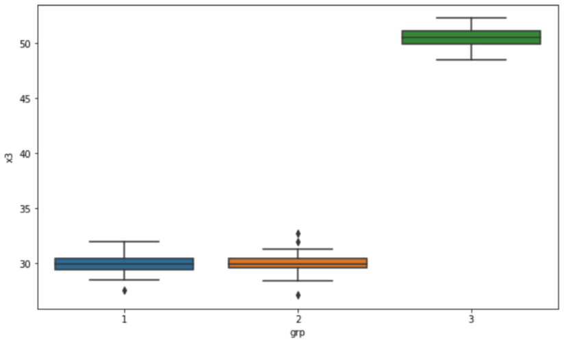
가령, 'x3' 변수에 대해 집단별로 상자 그래프 (Box plot for 'x3' by groups) 를 그려보면, 아래와 같이 집단1과 집단2는 유사한 반면에 집단3은 평균이 차이가 많이 나게 가상의 샘플 데이터가 생성되었음을 알 수 있습니다. 


## Boxplot for 'x3' by 'grp'
plt.rcParams['figure.figsize'] = [10, 6]
sns.boxplot(x='grp', y='x3', data=df)
plt.show()


여러개의 변수에 대해 일원분산분석을 하기 전에, 먼저 이해를 돕기 위해 Python의 statsmodels.api 모듈의 stats.anova_lm() 메소드를 사용해서 'x1' 변수에 대해 집단(집단 1/2/3)별로 평균이 같은지 일원분산분석으로 검정을 해보겠습니다. 


    - 귀무가설(H0) : 집단1의 x1 평균 = 집단2의 x1 평균 = 집단3의 x1 평균

    - 대립가설(H1) : 적어도 1개 이상의 집단의 x1 평균이 다른 집단의 평균과 다르다. (Not H0)


# ANOVA for x1 and grp
import statsmodels.api as sm
from statsmodels.formula.api import ols

model = ols('x1 ~ grp', data=df).fit()
sm.stats.anova_lm(model, typ=1)
[Out]

df	sum_sq	mean_sq	F	PR(>F)
grp	1.0	0.235732	0.235732	0.221365	0.639166
Residual	88.0	93.711314	1.064901	NaN	NaN


일원분산분석 결과 F 통계량이 0.221365, p-value가 0.639 로서 유의수준 5% 하에서 귀무가설을 채택합니다. 즉, 3개 집단 간 x1의 평균의 차이는 없다고 판단할 수 있습니다. (정규분포 X ~ N(0, 1) 를 따르는 모집단으로 부터 무작위로 3개 집단의 샘플을 추출했으므로 차이가 없게 나오는게 맞겠습니다.)


한개의 변수에 대한 일원분산분석하는 방법을 알아보았으니, 다음으로는 3개 집단별로 여러개의 연속형 변수인 'x1', 'x2', 'x3', 'x4' 에 대해서 for loop 순환문으로 돌아가면서 일원분산분석을 하고, 그 결과를 하나의 DataFrame에 모아보도록 하겠습니다. 


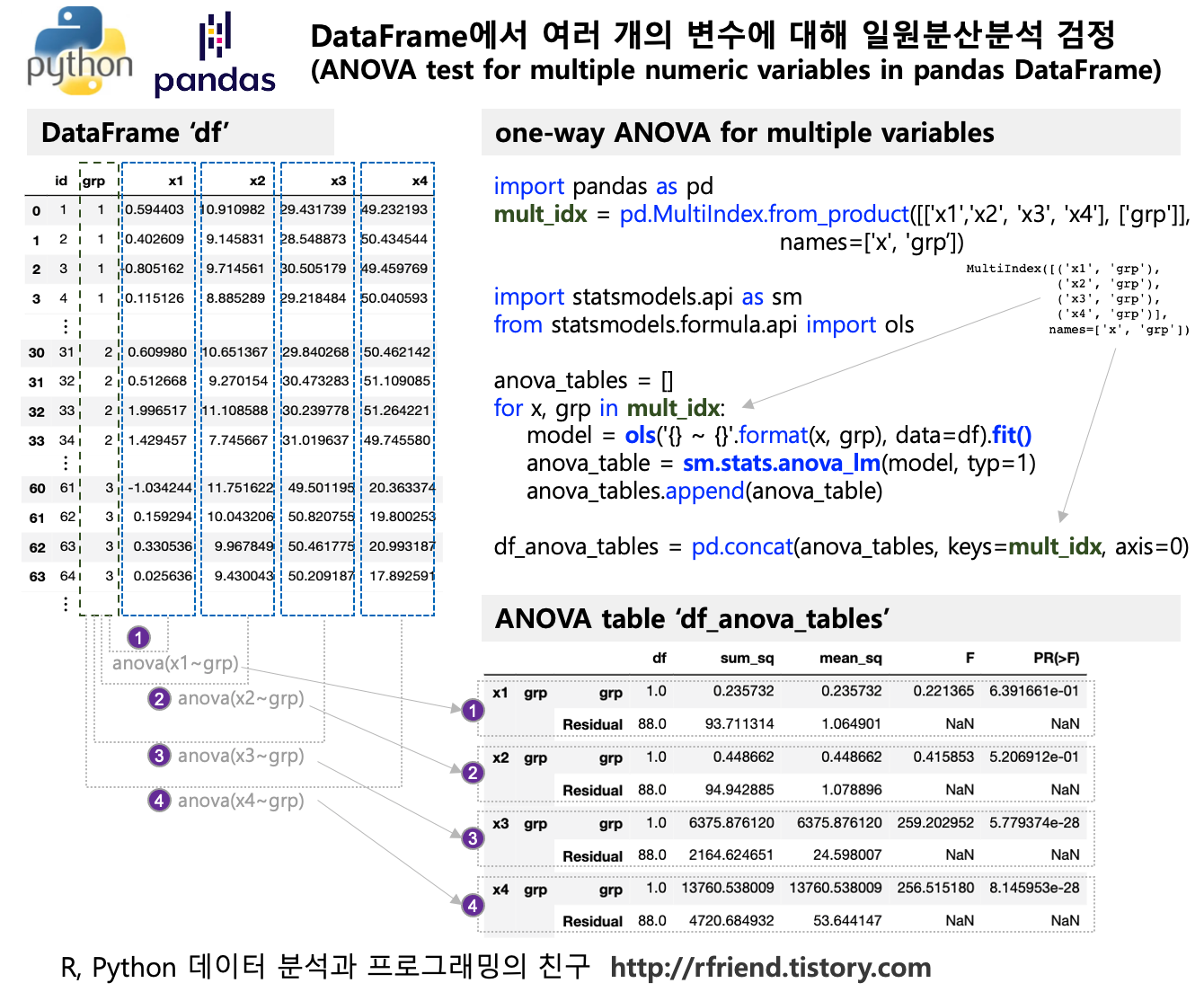
(1) 먼저, 일원분산분석을 하려는 모든 숫자형 변수와 집단 변수에 대한 가능한 조합의 MultiIndex 를 생성해줍니다. 


# make a multiindex for possible combinations of Xs and Group
num_col = ['x1','x2', 'x3', 'x4']
cat_col =  ['grp']
mult_idx = pd.MultiIndex.from_product([num_col, cat_col],
                                   names=['x', 'grp'])

print(mult_idx)
[Out]
MultiIndex([('x1', 'grp'),
            ('x2', 'grp'),
            ('x3', 'grp'),
            ('x4', 'grp')],
           names=['x', 'grp'])


(2) for loop 순환문(for x, grp in mult_idx:)으로 model = ols('{} ~ {}'.format(x, grp) 의 선형모델의  y, x 부분의 변수 이름을 바꾸어가면서 sm.stats.anova_lm(model, typ=1) 로 일원분산분석을 수행합니다. 이렇게 해서 나온 일원분산분석 결과 테이블을 anova_tables.append(anova_table) 로 순차적으로 append 해나가면 됩니다.  


# ANOVA test for multiple combinations of X and Group
import statsmodels.api as sm
from statsmodels.formula.api import ols

anova_tables = []
for x, grp in mult_idx:
    model = ols('{} ~ {}'.format(x, grp), data=df).fit()
    anova_table = sm.stats.anova_lm(model, typ=1)
    anova_tables.append(anova_table)

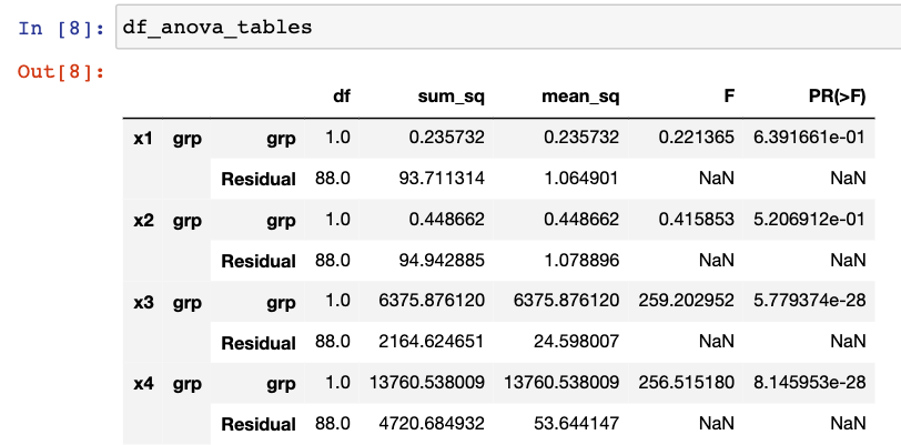
df_anova_tables = pd.concat(anova_tables, keys=mult_idx, axis=0)

df_anova_tables
[Out]

df	sum_sq	mean_sq	F	PR(>F)
x1	grp	grp	1.0	0.235732	0.235732	0.221365	6.391661e-01
Residual	88.0	93.711314	1.064901	NaN	NaN
x2	grp	grp	1.0	0.448662	0.448662	0.415853	5.206912e-01
Residual	88.0	94.942885	1.078896	NaN	NaN
x3	grp	grp	1.0	6375.876120	6375.876120	259.202952	5.779374e-28
Residual	88.0	2164.624651	24.598007	NaN	NaN
x4	grp	grp	1.0	13760.538009	13760.538009	256.515180	8.145953e-28
Residual	88.0	4720.684932	53.644147	NaN	NaN

anova tables


만약 특정 변수에 대한 일원분산분석 결과만을 조회하고 싶다면, 아래처럼 DataFrame의 MultiIndex 에 대해 인덱싱을 해오면 됩니다. 가령, 'x3' 에 대한 집단별 평균 차이 여부를 검정한 결과는 아래처럼 인덱싱해오면 됩니다. 


## Getting values of 'x3' from ANOVA tables
df_anova_tables.loc[('x3', 'grp', 'grp')]
[Out]

df         1.000000e+00
sum_sq     6.375876e+03
mean_sq    6.375876e+03
F          2.592030e+02
PR(>F)     5.779374e-28
Name: (x3, grp, grp), dtype: float64


F 통계량과 p-value 에 대해서 조회하고 싶으면 위의 결과에서 DataFrame 의 칼럼 이름으로 선택해오면 됩니다. 


# F-statistic
df_anova_tables.loc[('x3', 'grp', 'grp')]['F']
[Out]
259.2029515179077


# P-value
df_anova_tables.loc[('x3', 'grp', 'grp')]['PR(>F)']
[Out]
5.7793742588216585e-28


MultiIndex 를 인덱싱해오는게 좀 불편할 수 도 있는데요, 이럴 경우  df_anova_tables.reset_index() 로  MultiIndex 를 칼럼으로 변환해서 사용할 수도 있습니다. 

# resetting index to columns
df_anova_tables_2 = df_anova_tables.reset_index().dropna()


df_anova_tables_2
[Out]

level_0	level_1	level_2	df	sum_sq	mean_sq	F	PR(>F)
0	x1	grp	grp	1.0	0.235732	0.235732	0.221365	6.391661e-01
2	x2	grp	grp	1.0	0.448662	0.448662	0.415853	5.206912e-01
4	x3	grp	grp	1.0	6375.876120	6375.876120	259.202952	5.779374e-28
6	x4	grp	grp	1.0	13760.538009	13760.538009	256.515180	8.145953e-28


Greenplum DB에서 PL/Python (또는 PL/R)을 사용하여 여러개의 숫자형 변수에 대해 일원분산분석을 분산병렬처리하는 방법(one-way ANOVA in parallel using PL/Python on Greenplum DB)은 rfriend.tistory.com/640 를 참고하세요. 


[reference] 

* ANOVA test using Python statsmodels
 
: https://www.statsmodels.org/stable/generated/statsmodels.stats.anova.anova_lm.html


이번 포스팅이 많은 도움이 되었기를 바랍니다. 

행복한 데이터 과학자 되세요! :-)


728x90
반응형
Posted by Rfriend
,

2개의 모집단에 대한 평균을 비교, 분석하는 통계적 기법으로 t-Test를 활용하였다면, 비교하고자 하는 집단이 2개 이상일 경우에는 분산분석 (ANOVA : Analysis Of Variance)를 이용합니다. 


설명변수는 범주형 자료(categorical data)이어야 하며, 종속변수는 연속형 자료(continuous data) 일 때 2개 이상 집단 간 평균 비교분석에 분산분석(ANOVA) 을 사용하게 됩니다.


분산분석(ANOVA)은 기본적으로 분산의 개념을 이용하여 분석하는 방법으로서, 분산을 계산할 때처럼 편차의 각각의 제곱합을 해당 자유도로 나누어서 얻게 되는 값을 이용하여 수준평균들간의 차이가 존재하는 지를 판단하게 됩니다.  이론적인 부분에 대한 좀더 자세한 내용은 https://rfriend.tistory.com/131 를 참고하세요. 


one-way ANOVA  일원분산분석


이번 포스팅에서는 Python의  scipy 모듈의 stats.f_oneway() 메소드를 사용하여 샘플의 크기가 서로 다른 3개 그룹 간 평균에 차이가 존재하는지 여부를 일원분산분석(one-way ANOVA)으로 분석하는 방법을 소개하겠습니다. 


분산분석(Analysis Of Variance) 검정의 3가지 가정사항을 고려해서, 샘플 크기가 서로 다른 가상의 3개 그룹의 예제 데이터셋을 만들어보겠습니다. 


[ 분산분석  검정의 가정사항 (assumptions of ANOVA test) ]

  (1) 독립성: 각 샘플 데이터는 서로 독립이다. 
  (2) 정규성: 각 샘플 데이터는 정규분포를 따르는 모집단으로 부터 추출되었다. 
  (3) 등분산성: 그룹들의 모집단의 분산은 모두 동일하다. 


먼저, 아래의 예제 샘플 데이터셋은 그룹1과 그룹2의 평균은 '0'으로 같고, 그룹3의 평균은 '5'로서 나머지 두 그룹과 다르게 난수를 발생시켜 가상으로 만든 것입니다. 


# 3 groups of dataset with different sized samples 
import numpy as np
import pandas as pd
np.random.seed(1004)

data1 = np.random.normal(0, 1, 50)
data2 = np.random.normal(0, 1, 40)
data3 = np.random.normal(5, 1, 30) # different mean

data123 = [data1, data2, data3]


print(data123)
[Out]
[array([ 0.59440307,  0.40260871, -0.80516223,  0.1151257 , -0.75306522,
       -0.7841178 ,  1.46157577,  1.57607553, -0.17131776, -0.91448182,
        0.86013945,  0.35880192,  1.72965706, -0.49764822,  1.7618699 ,
        0.16901308, -1.08523701, -0.01065175,  1.11579838, -1.26497153,
       -1.02072516, -0.71342119,  0.57412224, -0.45455422, -1.15656742,
        1.29721355, -1.3833716 ,  0.3205909 , -0.59086187, -1.43420648,
        0.60998011,  0.51266756,  1.9965168 ,  1.42945668,  1.82880165,
       -1.40997132,  0.49433367,  0.9482873 , -0.35274099, -0.15359935,
       -1.18356064, -0.75440273, -0.85981073,  1.14256322, -2.21331694,
        0.90651805,  2.23629   ,  1.00743665,  1.30584548,  0.46669171]), array([-0.49206651, -0.08727244, -0.34919043, -1.11363541, -1.71982966,
       -0.14033817,  0.90928317, -0.60012686,  1.03906073, -0.03332287,
       -1.03424396,  0.15929405,  0.33053582,  0.02563551, -0.09213904,
       -0.91851177,  0.3099129 , -1.24211638, -0.33113027, -1.64086666,
       -0.27539834, -0.05489003,  1.50604364, -1.37756156, -1.25561652,
        0.16120867, -0.42121705,  0.2341905 , -1.20155195,  1.48131392,
        0.29105321,  0.4022031 , -0.41466037,  1.00502917,  1.45376705,
       -0.07038153,  0.52897801, -2.37895295, -0.75054747,  1.10641762]), array([5.91098191, 4.14583073, 4.71456131, 3.88528941, 5.23020779,
       5.12814125, 3.44610618, 5.36308351, 4.69463298, 7.49521024,
       5.41246681, 3.8724271 , 4.60265531, 4.60082925, 4.9074518 ,
       3.8141367 , 6.4457503 , 4.27553455, 3.63173152, 6.25540542,
       3.77536981, 7.19435668, 6.25339789, 6.43469547, 4.27431061,
       5.16694916, 7.21065725, 5.68274021, 4.81732021, 3.81650656])]


위의 3개 그룹의 커널밀도추정 그래프 (Kernel Density Estimates Plot)를 겹쳐서 그려보면, 아래와 같이 2개 집단은 서로 평균이 비슷하고 나머지 1개 집단은 평균이 확연히 다르다는 것을 직관적으로 알 수 있습니다. 

# Kernel Density Estimate Plot
import matplotlib.pyplot as plt
import seaborn as sns
plt.rcParams['figure.figsize'] = [10, 6]

sns.kdeplot(data1)
sns.kdeplot(data2)
sns.kdeplot(data3)
plt.show()


상자 그래프 (Box Plot) 으로 3개 집단 간 평균의 위치와 퍼짐 정도를 비교해보면, 역시 아래와 같이 그룹1과 그룹2는 서로 중심위치가 서로 비슷하고 그룹3만 중심위치가 확연히 다름을 알 수 있습니다. 


# Boxplot
sns.boxplot(data=data123)
plt.xlabel("Group", fontsize=14)
plt.ylabel("Value", fontsize=14)
plt.show()


이제 scipy 모듈의 scipy.stats.f_oneway() 메소드를 사용해서 서로 다른 개수의 샘플을 가진 3개 집단에 대해 평균의 차이가 존재하는지 여부를 일원분산분석을 통해 검정을 해보겠습니다. 


  - 귀무가설(H0): 3 집단의 평균은 모두 같다. (mu1 = mu2 = m3)

  - 대립가설(H1):  3 집단의 평균은 같지 않다.(적어도 1개 집단의 평균은 같지 않다) (Not H0)


F통계량은 매우 큰 값이고 p-value가 매우 작은 값이 나왔으므로 유의수준 5% 하에서 귀무가설을 기각하고 대립가설을 채택합니다. 즉, 3개 집단 간 평균의 차이가 존재한다고 평가할 수 있습니다

# ANOVA with different sized samples using scipy
from scipy import stats

stats.f_oneway(data1, data2, data3)
[Out] 
F_onewayResult(statistic=262.7129127080777, pvalue=5.385523527223916e-44)


F통계량과 p-value 를 각각 따로 따로 반환받을 수도 있습니다. 

# returning f-statistic and p-value
f_val, p_val = stats.f_oneway(*data123)

print('f-statistic:', f_val)
print('p-vale:', p_val)
[Out]
f-statistic: 262.7129127080777
p-vale: 5.385523527223916e-44


scipy 모듈의  stats.f_oneway() 메소드를 사용할 때 만약 데이터에 결측값(NAN)이 포함되어 있으면  'NAN'을 반환합니다. 위에서 만들었던 'data1'  numpy array 의 첫번째 값을  np.nan 으로 대체한 후에 scipy.stats.f_oneway() 로 일원분산분석 검정을 해보면  'NAN'(Not A Number)을 반환한 것을 볼 수 있습니다. 


# if there is 'NAN', then returns 'NAN'
data1[0] = np.nan
print(data1)
[Out]
array([        nan,  0.40260871, -0.80516223,  0.1151257 , -0.75306522,
       -0.7841178 ,  1.46157577,  1.57607553, -0.17131776, -0.91448182,
        0.86013945,  0.35880192,  1.72965706, -0.49764822,  1.7618699 ,
        0.16901308, -1.08523701, -0.01065175,  1.11579838, -1.26497153,
       -1.02072516, -0.71342119,  0.57412224, -0.45455422, -1.15656742,
        1.29721355, -1.3833716 ,  0.3205909 , -0.59086187, -1.43420648,
        0.60998011,  0.51266756,  1.9965168 ,  1.42945668,  1.82880165,
       -1.40997132,  0.49433367,  0.9482873 , -0.35274099, -0.15359935,
       -1.18356064, -0.75440273, -0.85981073,  1.14256322, -2.21331694,
        0.90651805,  2.23629   ,  1.00743665,  1.30584548,  0.46669171])

# returns 'nan'
stats.f_oneway(data1, data2, data3)
[Out] 
F_onewayResult(statistic=nan, pvalue=nan)


샘플 데이터에 결측값이 포함되어 있는 경우, 결측값을 먼저 제거해주고 일원분산분석 검정을 실시해주시기 바랍니다. 


# get rid of the missing values before applying ANOVA test
stats.f_oneway(data1[~np.isnan(data1)], data2, data3)
[Out]
F_onewayResult(statistic=260.766426640122, pvalue=1.1951277551195217e-43)


위의  일원분산분석(one-way ANOVA) 는 2개 이상의 그룹 간 평균의 차이가 존재하는지만을 검정할 뿐이며, 집단 간 평균의 차이가 존재한다는 대립가설을 채택하게 된 경우 어느 그룹 간 차이가 존재하는지는 사후검정 다중비교(post-hoc pair-wise multiple comparisons)를 통해서 알 수 있습니다. (rfriend.tistory.com/133)


pandas DataFrame 데이터셋에서 여러개의 숫자형 변수에 대해 for loop 순환문을 사용하여 집단 간 평균 차이 여부를 검정하는 방법은 rfriend.tistory.com/639 포스팅을 참고하세요. 


이번 포스팅이 많은 도움이 되었기를 바랍니다. 

행복한 데이터 과학자 되세요. 


[reference]

* scipy.stats.f_oneway : https://docs.scipy.org/doc/scipy/reference/generated/scipy.stats.f_oneway.html


scipy.stats.f_oneway — SciPy v1.6.3 Reference Guide

G.W. Heiman, “Understanding research methods and statistics: An integrated introduction for psychology”, Houghton, Mifflin and Company, 2001.

docs.scipy.org

728x90
반응형
Posted by Rfriend
,

이전 포스팅의  rfriend.tistory.com/262 에서는 Python pandas DataFrame의 결측값을 fillna() 메소드를 사용해서 특정 값으로 채우거나 평균으로 대체하는 방법을 소개하였습니다. 


이번 포스팅에서는 Python pandas DataFrame 의 결측값을 선형회귀모형(linear regression model) 을  사용하여 예측/추정하여 채워넣는 방법을 소개하겠습니다. (물론, 아래의 동일한 방법을 사용하여 선형회귀모형 말고 다른 통계, 기계학습 모형을 사용하여 예측/추정한 값으로 대체할 수 있습니다.)


(1) 결측값을 제외한 데이터로부터 선형회귀모형 훈련하기

    (training, fitting a linear regression model using non-missing values)

(2) 선형회귀모형으로 부터 추정값 계산하기 (prediction using linear regression model)

(3) pandas 의 fillna() 메소드 또는  numpy의  np.where()  메소드를 사용해서 결측값인 경우 선형회귀모형 추정값으로 대체하기 (filling missing values using the predicted values by linear regression model)


fill missing values of pandas DataFrame using predicted values by machine learning model


아래에는 예제로 사용할 데이터로 전복(abalone) 공개 데이터셋을 읽어와서 1행~3행의 'whole_weight' 칼럼 값을 결측값(NA) 으로 변환해주었습니다. 

import pandas as pd
import numpy as np

# read abalone dataset from website
abalone = pd.read_csv("http://archive.ics.uci.edu/ml/machine-learning-databases/abalone/abalone.data", 
                 header=None, 
                 names=['sex', 'length', 'diameter', 'height', 
                          'whole_weight', 'shucked_weight', 
                          'viscera_weight', 'shell_weight', 'rings'])
                          

# get 10 observations as an example
df = abalone.copy()[:10]


# check missing values : no missing value at all
pd.isnull(df).sum()
# sex               0
# length            0
# diameter          0
# height            0
# whole_weight      0
# shucked_weight    0
# viscera_weight    0
# shell_weight      0
# rings             0
# dtype: int64


# insert NA values as an example
df.loc[0:2, 'whole_weight'] = np.nan

df
# sex	length	diameter	height	whole_weight	shucked_weight	viscera_weight	shell_weight	rings
# 0	M	0.455	0.365	0.095	NaN	0.2245	0.1010	0.150	15
# 1	M	0.350	0.265	0.090	NaN	0.0995	0.0485	0.070	7
# 2	F	0.530	0.420	0.135	NaN	0.2565	0.1415	0.210	9
# 3	M	0.440	0.365	0.125	0.5160	0.2155	0.1140	0.155	10
# 4	I	0.330	0.255	0.080	0.2050	0.0895	0.0395	0.055	7
# 5	I	0.425	0.300	0.095	0.3515	0.1410	0.0775	0.120	8
# 6	F	0.530	0.415	0.150	0.7775	0.2370	0.1415	0.330	20
# 7	F	0.545	0.425	0.125	0.7680	0.2940	0.1495	0.260	16
# 8	M	0.475	0.370	0.125	0.5095	0.2165	0.1125	0.165	9
# 9	F	0.550	0.440	0.150	0.8945	0.3145	0.1510	0.320	19


(1) 결측값을 제외한 데이터로부터 선형회귀모형 훈련하기  (training, fitting a linear regression model using non-missing values)


 pandas 패키지의 dropna() 메소드를 이용해서 결측값이 포함된 행을 제거한 후의 설명변수  ' diameter', 'height', 'shell_weight' 를 'X' DataFrame 객체로 만들고, ' whole_weight' 를 종속변수  'y' Series로 만든 후에,  sklearn의  linear_model.LinearRegression() 메소드로   lin_reg.fit(X, y) 로 선형회귀모형을 적합하였습니다. 


# initiate sklearn's linear regression
from sklearn import linear_model

lin_reg = linear_model.LinearRegression()


# X and y after excluding missing values
X = df.dropna(axis=0)[['diameter', 'height', 'shell_weight']] 
y = df.dropna(axis=0)['whole_weight'] 


# fitting linear regression model using non-missing values
lin_reg_model = lin_reg.fit(X, y)


(2) 선형회귀모형으로 부터 추정값 계산하기 (prediction using linear regression model)


위의 (1)번에서 적합한 모델에 predict() 함수를 사용해서  'whole_weight'  의 값을 추정하였습니다. 


# Prediction
y_pred = lin_reg_model.predict(df.loc[:, ['diameter', 'height', 'shell_weight']])

y_pred
# array([0.54856977, 0.21868994, 0.69091523, 0.50734984, 0.19206521,
#        0.35618402, 0.80347213, 0.7804138 , 0.53164895, 0.85086606])


(3) pandas 의 fillna() 메소드 또는  numpy의  np.where()  메소드를 사용해서 결측값인 경우 선형회귀모형 추정값으로 대체하기 (filling missing values using the predicted values by linear regression model)


(방법 1)  pandas  의  fillna()  메소드를 사용해서  'whole_weight' 값이 결측값인 경우에는  위의 (2)번에서 선형회귀모형을 이용해 추정한 값으로 대체를 합니다. 이때  'y_pred' 는  2D numpy array 형태이므로, 이를 flatten() 메소드를 사용해서  1D array 로 바꾸어주고, 이를  pd.Series() 메소드를 사용해서 Series 데이터 유형으로 변환을 해주었습니다.   inplace=True 옵션을 사용해서 df DataFrame 내에서 결측값이 선형회귀모형 추정값으로 대체되고 나서 저장되도록 하였습니다. 


(방법 2)  numpy의 where() 메소드를 사용해서,  결측값인 경우  (즉,  isnull() 이 True)  pd.Series(y_pred.flatten()) 값을 가져옥, 결측값이 아닌 경우 기존 값을 가져와서  'whole_weight' 에 값을 할당하도록 하였습니다. 


(방법 3) for loop 을 돌면서 매 행의  'whole_weight' 값이 결측값인지 여부를 확인 후,  만약  결측값이면 (isnull() 이 True 이면) 위의 (1)에서 적합된 회귀모형에 X값들을 넣어줘서 예측을 해서 결측값을 채워넣는 사용자 정의함수를 만들고 이를  apply() 함수로 적용하는 방법도 생각해볼 수는 있으나, 데이터 크기가 큰 경우  for loop 연산은 위의 (방법 1), (방법 2) 의   vectorized operation 대비 성능이 많이 뒤떨어지므로 소개는 생략합니다. 


## filling missing values using predicted values by a linear regression model

## -- (방법 1) pd.fillna() methods
df['whole_weight'].fillna(pd.Series(y_pred.flatten()), inplace=True)


## -- (방법 2) np.where()
df['whole_weight'] = np.where(df['whole_weight'].isnull(), 
                              pd.Series(y_pred.flatten()), 
                              df['whole_weight'])
                              
## results
df
# sex	length	diameter	height	whole_weight	shucked_weight	viscera_weight	shell_weight	rings
# 0	M	0.455	0.365	0.095	0.548570	0.2245	0.1010	0.150	15
# 1	M	0.350	0.265	0.090	0.218690	0.0995	0.0485	0.070	7
# 2	F	0.530	0.420	0.135	0.690915	0.2565	0.1415	0.210	9
# 3	M	0.440	0.365	0.125	0.516000	0.2155	0.1140	0.155	10
# 4	I	0.330	0.255	0.080	0.205000	0.0895	0.0395	0.055	7
# 5	I	0.425	0.300	0.095	0.351500	0.1410	0.0775	0.120	8
# 6	F	0.530	0.415	0.150	0.777500	0.2370	0.1415	0.330	20
# 7	F	0.545	0.425	0.125	0.768000	0.2940	0.1495	0.260	16
# 8	M	0.475	0.370	0.125	0.509500	0.2165	0.1125	0.165	9
# 9	F	0.550	0.440	0.150	0.894500	0.3145	0.1510	0.320	19


많은 도움이 되었기를 바랍니다. 

행복한 데이터 과학자 되세요! :-)


728x90
반응형
Posted by Rfriend
,

이번 포스팅에서는 pandas DataFrame 의 칼럼 관련한 소소한 팁들을 정리해보았습니다. 


1. pandas DataFrame 의 칼럼 이름 확인 하기 : df.columns

2. pandas DataFrame 에 특정 칼럼 포함 여부 확인하기 : 'col' in df.columns

3. pandas DataFrame 에서 특정 칼럼 선택하기

4. pandas DataFrame 에서 특정 칼럼 제외하기

5. pandas DataFrame 칼럼 이름 바꾸기


pandas DataFrame column name list, check, difference, rename


먼저, 예제로 사용할 간단한 pandas DataFrame을 만들어보겠습니다. 


import pandas as pd

df = pd.DataFrame({'x1': [0.1, 0.1, 0.2, 0.2]
                   , 'x2': [10, 20, 30, 80]
                   , 'x3': [0.1, 0.3, 0.2, 0.6]
                   , 'y': [1, 2, 3, 10]}, 
                 index = [1, 2, 3, 4])
                 
df
[Out]:
    x1  x2   x3   y
1  0.1  10  0.1   1
2  0.1  20  0.3   2
3  0.2  30  0.2   3
4  0.2  80  0.6  10


1. pandas DataFrame 의 칼럼 이름 확인 하기 : df.columns

# DataFrame의 칼럼 이름 확인하기
df.columns

[Out]: Index(['x1', 'x2', 'x3', 'y'], dtype='object')


2. pandas DataFrame 에 특정 칼럼 포함 여부 확인하기 : 'col' in df.columns


'column_name' in df.columns 구문 형식으로 특정 칼럼이 포함되어있는지 여부를 True, False 의 boolean 형식으로 반환받을 수 있습니다.  이를 if 조건문과 함께 사용해서 특정 칼럼의 포함 여부에 따라 분기문을 만들 수 있습니다. 

# DataFrame의 칼럼 포함 여부 확인하기
'x1' in df.columns
[Out]: True


'x5' in df.columns
[Out]: False


if 'x1' in df.columns:
    print('column x1 is in df DataFrame')
[Out]: column x1 is in df DataFrame


3. pandas DataFrame 에서 특정 칼럼 선택하기


# 특정 칼럼 선택하기
y = df['y']

y
[Out]: 
1     1
2     2
3     3
4    10
Name: y, dtype: int64


# 여러개 칼럼 선택하기
X = df[['x1', 'x2', 'x3']]
X
[Out]:
        x1	x2	x3
1	0.1	10	0.1
2	0.1	20	0.3
3	0.2	30	0.2
4	0.2	80	0.6


4. pandas DataFrame 에서 특정 칼럼 제외하기


# 특정 칼럼 제외하고 나머지 칼럼 선택하기
X2 = df[df.columns.difference(['y'])]

X2
[Out]:
        x1	x2	x3
1	0.1	10	0.1
2	0.1	20	0.3
3	0.2	30	0.2
4	0.2	80	0.6


5. pandas DataFrame 칼럼 이름 바꾸기


# 칼럼 이름 바꾸기
X.columns = ['v1', 'v2', 'v3']

X
[Out]:

        v1	v2	v3
1	0.1	10	0.1
2	0.1	20	0.3
3	0.2	30	0.2
4	0.2	80	0.6


# 특정 칼럼만 선택해서 이름 바꾸기
X3 = X.rename(columns = {'v1': 'c1'})

X3
[Out]:
        c1	v2	v3
1	0.1	10	0.1
2	0.1	20	0.3
3	0.2	30	0.2
4	0.2	80	0.6


많은 도움이 되었기를 바랍니다. 

행복한 데이터 과학자 되세요! :-)


728x90
반응형
Posted by Rfriend
,

이전 포스팅에서는 numpy 배열의 원소 값을 사전(dictionary)의 (Key, Value)를 매핑해서 변환하는 방법을 소개하였습니다. (rfriend.tistory.com/620)


이번 포스팅에서는 Python numpy 의 array 배열의 순서대로 정수를 사전의 키(Key)로 하고, 배열 값을 사전의 값(Value)으로 하는 Python 사전(dictionary) 으로 변환하는 몇 가지 방법을 소개하겠습니다.


(1) dict() 와 enumerate() 함수를 이용해 배열로 부터 사전 만들기

(2) for loop 과 enumerate() 함수를 이용해 배열로 부터 사전 만들기


(1) dict() 와 enumerate() 함수를 이용해 배열로 부터 사전 만들기


먼저, numpy 라이브러리를 불러오고, 예제로 사용할 (5, 0) shape 의 numpy array 배열을 하나 만들어보겠습니다.


import numpy as np

cls_weight = np.array([0.30, 0.50, 0.10, 0.03, 0.07])
cls_weight
[Out]
array([0.3 , 0.5 , 0.1 , 0.03, 0.07])

cls_weight.shape
[Out] 
(5,)


위의 'cls_weight' 배열을 사전(dictionary)으로 변환해보겠습니다. 사전(dict) 키(Key)가 '0' 부터 시작하고, 배열의 순서대로 사전의 키가 하나씩 증가하며, 배열의 순서대로 사전에 값을 할당하여 보겠습니다.  dict() 함수는 객체를 '키(Key) : 값(Value)' 의 쌍을 가지는 사전형 자료구조를 만들어줍니다.


## converting numpy array to dictionary, 
## dict key is starting from 0
cls_weight_dict_from_0 = dict(enumerate(cls_weight))

cls_weight_dict_from_0
[Out]
{0: 0.3, 1: 0.5, 2: 0.1, 3: 0.03, 4: 0.07}


이때 dict() 안의 enumerate() 메소드는 객체를 순환할 때 회수를 세어주는 counter 를 같이 생성해서 enumerate 객체를 반환합니다. for loop 으로 enumerate 객체를 순환하면서 counter 와 배열 내 값을 차례대로 출력을 해보면 아래와 같습니다.

## enumerate() method adds a counter to an iterable 
## and returns it in a form of enumerate object
for i, j in enumerate(cls_weight):
    print(i, ':', j)
    
[Out]
0 : 0.3
1 : 0.5
2 : 0.1
3 : 0.03
4 : 0.07


경우에 따라서는 배열의 값으로 사전을 만들었을 때, 사전의 키 값이 '0'이 아니라 '1'이나 혹은 다른 숫자로 부터 시작하는 것을 원할 수도 있습니다. 이럴 경우 enumerate(iterable_object, 1) 처럼 원하는 숫자(아래 예에서는 '1')를 추가해주면 그 값이 더해져서 counter 가 생성이 됩니다.


## converting numpy array to dictionary, 
## dict key is starting from 1

cls_weight_dict_from_1 = dict(enumerate(cls_weight, 1))

cls_weight_dict_from_1
[Out]
{1: 0.3, 2: 0.5, 3: 0.1, 4: 0.03, 5: 0.07}


만약 사전(dictionary)으로 변환하려고 하는 numpy array의 axis 1의 축이 있다면 flatten() 메소드를 사용해서 axis 0 만 있는 배열로 먼저 평평하게 펴준 (axis 1 축을 없앰) 후에 위의 dict(enumerate()) 를 똑같이 사용해주면 됩니다.  아래 예는 shape (5, 1) 의 배열을 flatten() 메소드를 써서 shape (5, 0) 으로 바꿔준 후에 dict(enumerate()) 로 배열을 사전으로 변환해주었습니다.


## array with axis1
cls_weight_2 = np.array([[0.30], [0.50], [0.10], [0.03], [0.07]])
cls_weight_2
[Out]
array([[0.3 ],
       [0.5 ],
       [0.1 ],
       [0.03],
       [0.07]])


cls_weight_2.shape
[Out]
(5, 1)


## use flatten() method to convert shape (5, 1) to (5, 0)
cls_weight_dict_2 = dict(enumerate(cls_weight_2.flatten()))
print(cls_weight_dict_2)
[Out]
{0: 0.3, 1: 0.5, 2: 0.1, 3: 0.03, 4: 0.07}


(2) for loop 과 enumerate() 함수를 이용해 배열로 부터 사전 만들기


이번에는 for loop 과 enumerate() 메소드를 같이 이용하는 방법입니다. 위의 (1) 번 대비 좀 복잡한 느낌이 있기는 하지만, (1) 번 대비 (2) 방법은 for loop 안의 코드 블럭에 좀더 자유롭게 원하는 복잡한 로직을 녹여서 사전(dictionary)을 구성할 수 있다는 장점이 있습니다.


아래 예에서는 (a) 먼저 cls_weight_dict_3 = {} 로 비어있는 사전을 만들어 놓고, (b) for loop 으로 순환 반복을 하면서 enumerate(cls_weight) 가 반환해주는 (counter, 배열값) 로 부터 counter 정수 숫자를 받아서 cls_weight_dict_3 의 키(Key) 로 할당해주고, 배열의 값을 사전의 해당 키에 할당해주는 방식입니다.  사전의 키에 값 할당(assinging Value to dict by mapping Key)은 Dict[Key] = Value 구문으로 해줍니다.


cls_weight = np.array([0.30, 0.50, 0.10, 0.03, 0.07])
cls_weight
[Out]
array([0.3 , 0.5 , 0.1 , 0.03, 0.07])

## Converting a numpy array to a dictionary
## Dict key is starting from 0
cls_weight_dict_3 = {}

for i, c_w in enumerate(cls_weight):
    cls_weight_dict_3[i] = c_w
    

print(cls_weight_dict_3)
[Out]
{0: 0.3, 1: 0.5, 2: 0.1, 3: 0.03, 4: 0.07}


사전의 키를 '0' 이 아니라 '1'부터 시작하게 하려면 enumerate()의 counter가 0부터 시작하므로, counter를 사전의 키에 할당할 때 'counter+1' 을 해주면 됩니다.


## converting a numpy array to a dictionary using for loop
## dict key is strating from 1

## null dict
cls_weight_dict_3_from_1 = {}

## assigning values by keys + 1
for i, c_w in enumerate(cls_weight):
    cls_weight_dict_3_from_1[i+1] = c_w
    
    
print(cls_weight_dict_3_from_1)
[Out]
{1: 0.3, 2: 0.5, 3: 0.1, 4: 0.03, 5: 0.07}


이번 포스팅이 많은 도움이 되었기를 바랍니다.

행복한 데이터 과학자 되세요! :-)


728x90
반응형
Posted by Rfriend
,

이번 포스팅에서는 1차원 배열 내 고유한 원소 집합 (a set with unique elements) 을 찾고, 더 나아가서 고유한 원소별 개수(counts per unique elements)도 세어보고, 원소 개수를 기준으로 정렬(sorting)도 해보는 여러가지 방법을 소개하겠습니다.


(1) numpy 1D 배열 안에서 고유한 원소 집합 찾기
    (finding a set with unique elements in 1D numpy array)

(2) numpy 1D 배열 안에서 고유한 원소 별로 개수 구하기
    (counts per unique elements in 1D numpy array)

(3) numpy 1D 배열 안에서 고유한 원소(key) 별 개수(value)를 사전형으로 만들기

    (making a dictionary with unique sets and counts of 1D numpy array)

(4) numpy 1D 배열의 고유한 원소(key) 별 개수(value)의 사전을 정렬하기

    (sorting a dictionary with unique sets and counts of 1D numpy array)

(5) numpy 1D 배열을 pandas Series 로 변환해서 고유한 원소 별 개수 구하고 정렬하기

    (converting 1D array to pandas Series, and value_counts(), sort_values())

(6) numpy 1D 배열을 pandas DataFrame으로 변환해 고유 원소별 개수 구하고 정렬하기

    (converting 1D array to pandas DataFrame, and value_counts(), sort_values())


먼저, 예제로 사용할 간단한 numpy 1D 배열을 만들어보겠습니다.


## simple 1D numpy array

import numpy as np

arr = np.array(['a', 'c', 'c', 'b', 'a', 
                'b', 'b', 'c', 'a', 'c', 
                'b', 'a', 'a', 'a', 'c'])
                
                
arr
[Out] array(['a', 'c', 'c', 'b', 'a', 'b', 'b', 'c', 'a', 'c', 
             'b', 'a', 'a', 'a', 'c'], dtype='<U1')


(1) numpy 1D 배열 안에서 고유한 원소 집합 찾기
    (finding a set with unique elements in 1D numpy array)


np.unique() 메소드를 사용하면 numpy 배열 내 고유한 원소(unique elements)의 집합을 찾을 수 있습니다.


## np.unique(): Find the unique elements of an array
np.unique(arr)
[Out] 
array(['a', 'b', 'c'], dtype='<U1')


더 나아가서, return_inverse=True 매개변수를 설정해주면, 아래의 예처럼 numpy 배열 내 고유한 원소의 집합 배열과 함께 '고유한 원소 집합 배열의 indices 의 배열' 을 추가로 반환해줍니다.

따라서 이 기능을 이용하면 array(['a', 'c', 'c', 'b', 'a', 'b', 'b', 'c', 'a', 'c', 'b', 'a', 'a', 'a', 'c']) 를 ==> array([0, 2, 2, 1, 0, 1, 1, 2, 0, 2, 1, 0, 0, 0, 2]) 로 쉽게 변환할 수 있습니다.


## return_inverse=True: If True, also return the indices of the unique array
np.unique(arr, 
          return_inverse=True)
[Out]
(array(['a', 'b', 'c'], dtype='<U1'),
 array([0, 2, 2, 1, 0, 1, 1, 2, 0, 2, 1, 0, 0, 0, 2]))


(2) numpy 1D 배열 안에서 고유한 원소 별로 개수 구하기
    (counts per unique elements in 1D numpy array)


위의 (1)번에서 np.unique() 로 numpy 배열 내 고유한 원소의 집합을 찾았다면, return_counts = True 매개변수를 설정해주면 각 고유한 원소별로 개수를 구해서 배열로 반환할 수 있습니다.


## return_counts: If True, also return the number of times each unique item appears in ar.
np.unique(arr, 
          return_counts = True)     

[Out]
(array(['a', 'b', 'c'], dtype='<U1'), array([6, 4, 5]))


(3) numpy 1D 배열 안에서 고유한 원소(key) 별 개수(value)를 사전형으로 만들기

    (making a dictionary with unique sets and counts of 1D numpy array)


위의 (2)번에서 각 고유한 원소별 개수를 구해봤는데요, 이를 파이썬의 키:값 쌍 (key: value pair) 형태의 사전(dictionary) 객체로 만들어보겠습니다.


먼저 np.unique(arr, return_counts = True) 의 결과를 unique, counts 라는 이름의 array로 할당을 받고, 이를 zip(unique, counts) 으로 쌍(pair)을 만들어준 다음에, dict() 를 사용해서 사전형으로 변환해주었습니다.


## making a dictionary with unique elements and counts of 1D array
unique, counts = np.unique(arr, return_counts = True)
uniq_cnt_dict = dict(zip(unique, counts))

uniq_cnt_dict
[Out]
{'a': 6, 'b': 4, 'c': 5}


(4) numpy 1D 배열의 고유한 원소(key) 별 개수(value)의 사전을 정렬하기

    (sorting a dictionary with unique sets and counts of 1D numpy array)


위의 (3)번까지 잘 진행을 하셨다면 이제 (unique : counts) 쌍의 사전을 'counts' 의 값을 기준으로 오름차순 정렬(sorting a dict by value in ascending order) 또는 내림차순 정렬 (sorting a dict by value in descending order) 하고 싶은 마음이 생길 수 있는데요, 이럴 경우 sorted() 메소드를 사용하면 되겠습니다. (pytho dictionary 정렬 참조: rfriend.tistory.com/473)


## sorting a dictionary by value in ascending order
## -- reference: https://rfriend.tistory.com/473
sorted(uniq_cnt_dict.items(), 
       key = lambda x: x[1])
       
[Out]
[('b', 4), ('c', 5), ('a', 6)]


## sorting a dictionary by value in descending order
sorted(uniq_cnt_dict.items(), 
       reverse = True, 
       key = lambda x: x[1])
       
[Out]
[('a', 6), ('c', 5), ('b', 4)]


(5) numpy 1D 배열을 pandas Series 로 변환해 고유한 원소별 개수 구하고 정렬하기

    (converting 1D array to pandas Series, and value_counts(), sort_values())


pandas 의 Series 나 DataFrame으로 변환해서 데이터 분석 하는 것이 더 익숙하거나 편리한 상황에서는 pandas.Series(array) 나 pandas.DataFrame(array) 로 변환을 해서, value_count() 메소드로 원소의 개수를 세거나, sort_values() 메소드로 값을 기준으로 정렬을 할 수 있습니다.


import pandas as pd

## converting an array to pandas Series
arr_s = pd.Series(arr)
arr_s
[Out]
0     a
1     c
2     c
3     b
4     a
5     b
6     b
7     c
8     a
9     c
10    b
11    a
12    a
13    a
14    c
dtype: object


## counting values by unique elements of pandas Series
arr_s.value_counts()
[Out]
a    6
c    5
b    4
dtype: int64


## sorting by values in ascending order of pandas Series
arr_s.value_counts().sort_values(ascending=True)
[Out]
b    4
c    5
a    6
dtype: int64


(6) numpy 1D 배열을 pandas DataFrame으로 변환해 고유한 원소별 개수 구하고 정렬하기

    (converting 1D array to pandas DataFrame, and value_counts(), sort_values())


만약 pandas Series 내 고유한 원소별 개수를 구한 결과를 개수의 오름차순으로 정렬을 하고 싶다면 sort_values(ascending = True) 를 설정해주면 됩니다. (내림차순이 기본 설정, default to descending order)


import pandas as pd

## converting an array to pandas DataFrame
arr_df = pd.DataFrame(arr, columns=['x1'])
arr_df

[Out]
x1
0	a
1	c
2	c
3	b
4	a
5	b
6	b
7	c
8	a
9	c
10	b
11	a
12	a
13	a
14	c


## counting the number of unique elements in Series
arr_df['x1'].value_counts()
[Out]
a    6
c    5
b    4
Name: x1, dtype: int64


## # sorting by the counts of unique elements in ascending order
arr_df['x1'].value_counts().sort_values(ascending=True)
[Out]
b    4
c    5
a    6
Name: x1, dtype: int64


이번 포스팅이 많은 도움이 되었기를 바랍니다.

행복한 데이터 과학자 되세요!  :-)


728x90
반응형
Posted by Rfriend
,

이번 포스팅에서는 Python numpy 의 배열의 원소 값을 사전(dictionary)의 {키: 값} 쌍 ({key: value} pair) 을 이용해서, 배열의 원소 값과 사전의 키를 매핑하여 사전의 값으로 배열의 원소값을 변환하는 방법을 소개하겠습니다.


아래의 예에서는 다중분류 (multi-class classification) 기계학습 모델로 부터 각 관측치가 5개 classes 별 속할 확률을 배열로 반환받은 상황을 가정하여 만들어보았습니다.


(1) 다중분류 확률 배열로 부터 최대값의 위치 인덱스 가져오기

(2) np.vectorize() 와 dict.get() 을 사용해서 최대값 위치 인덱스와 분류 레이블을 매핑하기

(3) for loop 과 dict.get() 을 사용해서 최대값 위치 인덱스와 분류 레이블을 매핑하기


(1) 다중분류 확률 배열로 부터 최대값의 위치 인덱스 가져오기


먼저, 5개 class를 가지는 다중분류 문제에서 5개 class 별 속할 확률을 기계학습 분류 모델로 부터 아래의 'pred_proba' 라는 이름의 배열로 얻었다고 가정해보겠습니다.


import numpy as np

## probability for each classes
pred_proba = np.array([[0., 0., 0.2, 0.8, 0.], 
                       [0.9, 0., 0., 0., 0.1], 
                       [0., 0., 0.6, 0.2, 0.2], 
                       [0., 0., 0.5, 0.3, 0.2], 
                       [0., 0.1, 0.3, 0., 0.6], 
                       [0., 0.4, 0., 0.3, 0.3]])

pred_proba
[Out]
array([[0. , 0. , 0.2, 0.8, 0. ],
       [0.9, 0. , 0. , 0. , 0.1],
       [0. , 0. , 0.6, 0.2, 0.2],
       [0. , 0. , 0.5, 0.3, 0.2],
       [0. , 0.1, 0.3, 0. , 0.6],
       [0. , 0.4, 0. , 0.3, 0.3]])


이들 확률값 배열로 부터 하나의 예측값을 구하기 위해 이들 5개 각 class별 확률 중에서 가장 큰 값을 가지는 위치 (indices of maximum value) 의 class 를 모델이 예측한 class 라고 정의해보겠습니다.  

np.argmax(pred_proba, axis=1) 은 배열 내의 각 관측치 별 (axis = 1) 로 가장 큰 확률값의 위치의 인덱스를 반환합니다.  가령, 위의 pred_proba 의 첫번째 관측치의 5개 class 별 속할 확률은 [0., 0., 0.2, 0.8, 0.] 의 배열로서, 확률 0.8 이 가장 큰 값이므로 위치 인덱스 '3'을 반환하였습니다.


## positional index for maximum probability
pred_idx = np.argmax(pred_proba, axis=1)
pred_idx
[Out]
array([3, 0, 2, 2, 4, 1])


(2) np.vectorize() 와 dict.get() 을 사용해서 최대값 위치 인덱스와 분류 레이블을 매핑하기


위의 (1)번에서 구한 확률 최대값의 위치 인덱스 가지고, 이번에는 아래의 'class_map_dict'와 같이 {키: 값} 쌍 사전의 '키(key)'를 기준으로 매핑을 해서, 다중분류 모델의 예측값을 'class 이름'으로 변환을 해보겠습니다.


## dictionary with pairs of {index_max_proba: class_name}
class_map_dict = {
    0: 'noraml', 
    1: 'class01', 
    2: 'class02', 
    3: 'class03',
    4: 'class04'
}

class_map_dict
[Out]
{0: 'noraml', 1: 'class01', 2: 'class02', 3: 'class03', 4: 'class04'}


이때 dict.get(key) 를 유용하게 사용할 수 있습니다. dict.get(key) 메소드는 사전(dict)의 키에 쌍으로 대응하는 값을 반환해줍니다. 따라서 바로 위에서 정의해준 'class_map_dict'의 키 값을 넣어주면, 각 키에 해당하는 'normal'~'class04' 의 사전 값을 반환해줍니다.


## get() returns the value for the specified key if key is in dict.
class_map_dict.get(pred_idx[0])
[Out]
'class03'


class_map_dict.get(0)
[Out]
'noraml'


사전의 (키: 값)을 매핑하려는 배열 내 원소가 많을 경우, np.vectorize() 메소드를 이용하면 매우 편리하고 또 빠르게 사전의 (키: 값)을 매핑을 해서 배열의 값을 변환할 수 있습니다. 아래 예에서는 'class_map_dict' 의 (키: 값) 사전을 사용해서 'pred_idx'의 확률 최대값 위치 인덱스 배열을 'pred_cls' 의 예측한 클래스(레이블) 이름('normal'~'class04')으로 변환해주었습니다.


np.vectorize() 는 numpy의 broadcasting 규칙을 사용해서 매핑을 하므로 코드가 깔끔하고, for loop을 사용하지 않으므로 원소가 많은 배열을 처리해야 할 경우 빠릅니다.


## vectorization of dict.get(array_idx) for all elements of array
pred_cls = np.vectorize(class_map_dict.get)(pred_idx)

pred_cls
[Out]
array(['class03', 'noraml', 'class02', 'class02', 'class04', 'class01'],
      dtype='<U7')
      

* np.vectorize() reference: numpy.org/doc/stable/reference/generated/numpy.vectorize.html


(3) for loop 과 dict.get() 을 사용해서 최대값 위치 인덱스와 분류 레이블을 매핑하기


만약 위의 (2)번 처럼 np.vectorize() 메소드를 사용하지 않는다면, 아래처럼 for loop 사용해서 확률 최대값 위치 인덱스의 개수 만큼 순환 반복을 하면서 dict.get() 함수를 적용해주어야 합니다. 위의 (2)번 대비 코드도 길고, 또 대상 배열이 클 경우 시간도 더 오래 걸리므로 np.vectorize() 사용을 권합니다.


## manually using for loop
pred_cls_mat = np.empty(pred_idx.shape, dtype='object')

for i in range(len(pred_idx)):
    pred_cls_mat[i] = class_map_dict.get(pred_idx[i])
    
pred_cls_mat
[Out]
array(['class03', 'noraml', 'class02', 'class02', 'class04', 'class01'],
      dtype=object)


이번 포스팅이 많은 도움이 되었기를 바랍니다.

행복한 데이터 과학자 되세요!  :-)


728x90
반응형
Posted by Rfriend
,

Python pandas에는 DataFrame 내 숫자형 변수의 결측값 여부를 확인(rfriend.tistory.com/260)하거나 결측값을 채우는(rfriend.tistory.com/262) 다양하고 간단한 함수를 제공합니다.


이번 포스팅에서는 범주형 자료의 결측값을 각 범주별 구성비율에 비례하여 확률적으로 채우는 방법을 소개하겠습니다. 가령, 'A' 범주가 50%, 'B' 범주가 30%, 'C' 범주가 20%를 구성하고 있으며, 결측값 발생 시 각 범주별 구성비율에 따라서 확률적으로 결측값을 채워넣어보겠습니다.

(엄밀히 말하면 공백 '', '   ' 나 'None' 등은 결측값이라고 말하기 곤란합니다만... 문자열 '' 을 결측값이라고 정의하겠습니다.) 


댓글로 위의 요건을 수행하는 Python 코드에 대한 질문을 남겨주신 분이 계셔서 그때 답변 달았던 내용을 포스팅으로 옮겨보았습니다.


절차는 2단계로 이루어집니다.


(1) 균등분포(uniform distribution)로 부터 난수를 생성하여 각 범주의 구성비율에 따라 결측값을 채우는 값을 지정하는 사용자 정의 함수 생성

(2) for loop 반복문으로 범주형 변수의 결측값일 경우 (1)번 사용자 정의 함수를 실행하여 결측값 채우기


먼저, 예제로 사용할 문자열로 구성된 칼럼에 결측값('')을 가진 간단한 DataFrame을 만들어보겠습니다.


## DataFrame with missing value in categorical variable
import pandas as pd

df = pd.DataFrame({'x1': ['A', 'A', 'C', '', 'A', 'B', 'A', 'B', 'A', 'A', 
                          'C', '', 'A', 'A', '', 'A', 'B', 'A', 'C', 'A', '']})
                          
print(df)
[Out]
   x1
0   A
1   A
2   C
3      <-- missing
4   A
5   B
6   A
7   B
8   A
9   A
10  C
11     <-- missing
12  A
13  A
14     <-- missing
15  A
16  B
17  A
18  C
19  A
20     <-- missing
20   


(1) 균등분포(uniform distribution)로 부터 난수를 생성하여 각 범주의 구성비율에 따라 결측값을 채우는 값을 지정하는 사용자 정의 함수 생성


균등분포(uniform distribution)는 구간 [min, max] 에서 값이 균등하게 퍼져있는 집단, 일어날 확률이 균등한 분포를 말합니다. 가령, 구간 [0, 1] 에서 임의로 난수를 생성할 경우 그 값이 뽑힐 확률은 모두 1로서 동일하게 됩니다. (만약 구간 [0, 10] 에서 난수를 생성할 경우 각 값이 뽑힐 확률은 모두 0.1로서 동일하게 됨).


numpy 의 random.uniform(min, max, size) 메소드를 사용해서 균등분포로 부터 난수를 생성할 수 있습니다. 아래는 구간 [0. 1] 에서 난수 10개를 생성한 예입니다.


import numpy as np

np.random.uniform(0, 1, 10)

[Out]
array([0.56947875, 0.95692566, 0.9978566 , 0.99739644, 0.00885555,
       0.92047312, 0.00443685, 0.12121749, 0.46886965, 0.32319941])


그럼, 이제 모집단에서 각 범주가 차지하는 비율이 'A' 범주(category, class)는 50%, 'B' 범주는 30%, 'C' 범주는 20%라고 하고, 이 각 범주별 구성비율에 비례해서 범주의 결측치를 확률적으로, 임의로 채우는 사용자 정의 함수를 정의해보겠습니다.


## 'A' 0.5 : 'B' 0.3 : 'C' 0.2
def cat_fill_na():
    # generate random number from uniform distrubution
    rnd_num = np.random.uniform(0, 1, 1)
    
    if rnd_num > 0.8:
        x = 'C'
    elif rnd_num > 0.5:
        x = 'B'
    else:
        x = 'A'
    
    return x


(2) for loop 반복문으로 범주형 변수의 결측값일 경우 (1)번 사용자 정의 함수를 실행하여 결측값 채우기 


이제 위의 (1)번에서 정의한 사용자 정의 함수를 사용해서 범주형 변수의 관측치들 중에서 결측값('')의 경우 확률적으로 범주 값을 채워넣어보겠습니다.

for i in range(df.shape[0]):
    if df['x1'].iloc[i] == '':
        df['x1'].iloc[i] = cat_fill_na
        
df
[Out]
x1
0	A
1	A
2	C
3	C  <-- filled randomly with probability of ('A' 50%, 'B' 30%, 'C' 20%)
4	A
5	B
6	A
7	B
8	A
9	A
10	C
11	C  <-- filled randomly with probability of ('A' 50%, 'B' 30%, 'C' 20%)
12	A
13	A
14	C  <-- filled randomly with probability of ('A' 50%, 'B' 30%, 'C' 20%)
15	A
16	B
17	A
18	C
19	A
20	B  <-- filled randomly with probability of ('A' 50%, 'B' 30%, 'C' 20%)


---------------------------------------------------------------------------------------------

참고로, 아래처럼 코드를 수행하면 단 한번만 균등분포로부터 난수를 발생하여 해당 난수값이 포함된 단 하나의 범주값을 모든 결측값에 채워넣게 되므로 이번 요건에는 적합하지 않습니다.


## define UDF
def cat_fill_na(x):
    if x == '':
        rnd_int = random.randint(1, 10)
        if rnd_int == 9:
            x = 'B'
        elif rnd_int == 10:
            x = 'C'
        else:
            x = 'A'
    else:
        x = x
        
    return x
    
## run UDF    
df2 = df.apply(lambda x: cat_fill_na(x['x1']), axis=1)

df2
0     A
1     A
2     C
3     A  <-- filled with the same value
4     A
5     B
6     A
7     B
8     A
9     A
10    C
11    A   <-- filled with the same value
12    A
13    A
14    A   <-- filled with the same value
15    A
16    B
17    A
18    C
19    A
20    A   <-- filled with the same value
dtype: object


이번 포스팅이 많은 도움이 되었기를 바랍니다.

행복한 데이터 과학자 되세요!  :-)


728x90
반응형
Posted by Rfriend
,

이전 포스팅에서는 무작위(확률, 임의) 표본 추출과 관련하여,

- numpy.random() 메소드를 이용하여 확률분포별 확률 표본 추출, 난수 생성: https://rfriend.tistory.com/284

- 그룹별 무작위 표본 추출: https://rfriend.tistory.com/407

- 기계학습을 위한 Train, Test 데이터셋 분할: https://rfriend.tistory.com/519

- 층화 무작위 추출을 통한 Train, Test 데이터셋 분할: https://rfriend.tistory.com/520

방법에 대하여 소개하였습니다.


이번 포스팅에서는 Python pandas 모듈의 DataFrame.sample() 메소드를 사용해서 DataFrame으로 부터 무작위 (확률, 임의) 표본 추출 (random sampling) 하는 방법을 소개하겠습니다.


(1) DataFrame으로 부터 특정 개수의 표본을 무작위로 추출하기 (number)

(2) DataFrame으로 부터 특정 비율의 표본을 무작위로 추출하기 (fraction)

(3) DataFrame으로 부터 복원 무작위 표본 추출하기 (random sampling with replacement)

(4) DataFrame으로 부터 가중치를 부여하여 표본 추출하기 (weights)

(5) DataFrame으로 부터 칼럼에 대해 무작위 표본 추출하기 (axis=1, axis='column)

(6) DataFrame으로 부터 특정 칼럼에 대해 무작위 표본 추출한 결과를 numpy array로 할당하기


[ pandas DataFrame에서 무작위 (확률) 표본 추출하기: pandas.DataFrame.sample() ]


  (1) DataFrame으로 부터 특정 개수의 표본을 무작위(확률)로 추출하기 (number)


예제로 사용할 4개의 관측치와 3개의 칼럼을 가진 pandas DataFrame을 만들어보겠습니다.

(참조 [1] 의 pandas tutorial 코드 사용하였습니다.)


import pandas as pd

df = pd.DataFrame({'num_legs': [2, 4, 8, 0],
                   'num_wings': [2, 0, 0, 0],
                   'num_specimen_seen': [10, 2, 1, 8]},
                  index=['falcon', 'dog', 'spider', 'fish'])

df


num_legsnum_wingsnum_specimen_seen
falcon2210
dog402
spider801
fish008


DataFrame.sample() 메소드의 n 매개변수를 사용해서 특정 개수 (number)의 표본을 무작위로 추출할 수 있습니다. 그리고 random_state 매개변수는 무작위(확률) 표본 추출을 위한 난수(random number)를 생성할 때 초기값(seed number) 로서, 재현가능성(reproducibility)을 위해서 설정해줍니다.


아래 예에서는 총 4개 관측치 중에서 2개의 관측치 (n=2) 를 무작위 표본 추출해보았습니다. Index를 기준으로 n 개수 만큼 표본을 추출해서 모든 칼럼의 값을 pandas DataFrame 자료구조로 반환합니다.


df.sample(n=2, # number of items from axis to return.
          random_state=1004) # seed for random number generator for reproducibility


num_legsnum_wingsnum_specimen_seen
falcon2210
fish008


  (2) DataFrame으로 부터 특정 비율의 표본을 무작위로 추출하기 (fraction)


DataFrame으로 부터 특정 비율(fraction)으로 무작위 표본 추출을 하고 싶으면 frac 매개변수에 0~1 사이의 부동소수형(float) 값을 입력해주면 됩니다.


df.sample(frac=0.5, # fraction of axis items to return.
          random_state=1004)


num_legsnum_wingsnum_specimen_seen
falcon2210
fish008


만약 비복원 추출 모드 (replace = False, 기본 설정) 에서 frac 값이 1을 초과할 경우에는 "ValueError: Replace has to be set to 'True' when upsampling the population 'frac' > 1." 이라는 에러가 발생합니다. 왜냐하면 모집단의 표본 개수 (100%, frac=1) 보다 더 많은 표본을 비복원 추출로는 할 수 없기 때문입니다. (복원 추출의 경우 동일한 관측치를 다시 표본 추출할 수 있으므로 frac > 1 인 경우도 가능함.)


## ValueError: Replace has to be set to `True` when upsampling the population `frac` > 1.
df.sample(frac=1.5,
          random_state=1004)


---------------------------------------------------------------------------
ValueError                                Traceback (most recent call last)
<ipython-input-45-2fcc4494d7ae> in <module>
----> 1 df.sample(frac=1.5, # fraction of axis items to return. 
      2           random_state=1004)

~/opt/anaconda3/lib/python3.8/site-packages/pandas/core/generic.py in sample(self, n, frac, replace, weights, random_state, axis)
   5326             n = 1
   5327         elif frac is not None and frac > 1 and not replace:
-> 5328             raise ValueError(
   5329                 "Replace has to be set to `True` when "
   5330                 "upsampling the population `frac` > 1."

ValueError: Replace has to be set to `True` when upsampling the population `frac` > 1.


만약 DataFrame.sample() 메소드에서 표본 개수 n 과 표본추출 비율 frac 을 동시에 설정하게 되면 "ValueError: Please enter a value for 'frac' OR 'n', not both" 에러가 발생합니다. n 과 frac 둘 중에 하나만 입력해야 합니다.


## parameter 'n' and 'frac' cannot be used at the same time.
## ValueError: Please enter a value for `frac` OR `n`, not both
df.sample(n=2, frac=0.5)


---------------------------------------------------------------------------
ValueError                                Traceback (most recent call last)
<ipython-input-6-b31ebc150882> in <module>
      1 ## parameter 'n' and 'frac' cannot be used at the same time.
      2 ## ValueError: Please enter a value for `frac` OR `n`, not both
----> 3 df.sample(n=2, frac=0.5)

~/opt/anaconda3/lib/python3.8/site-packages/pandas/core/generic.py in sample(self, n, frac, replace, weights, random_state, axis)
   5335             n = int(round(frac * axis_length))
   5336         elif n is not None and frac is not None:
-> 5337             raise ValueError("Please enter a value for `frac` OR `n`, not both")
   5338 
   5339         # Check for negative sizes

ValueError: Please enter a value for `frac` OR `n`, not both


  (3) DataFrame으로 부터 복원 무작위 표본 추출하기

      (random sampling with replacement)


한번 추출한 표본을 다시 모집단에 되돌려 넣고 추출하는 방법을 복원 추출법 (sampling with replacement) 이라고 합니다. 복원 추출법을 사용하면 동일한 표본이 중복해서 나올 수 있습니다.


DataFrame.sample() 메소드에서는 repalce=True 로 설정하면 복원 추출을 할 수 있습니다. 많은 경우 한번 추출된 표본은 되돌려 놓지 않고 표본을 추출하는 비복원 추출(sampling without replacement)을 사용하며, 기본 설정은 replace=False 입니다.


## replace=True: random sampling with replacement
df.sample(n=8, # or equivalently: frac=2
          replace=True, # random sampling with replacement
          random_state=1004)


num_legsnum_wingsnum_specimen_seen
spider801
fish008
fish008
dog402
fish008
fish008
fish008
spider801


만약 비복원 추출 모드 (replace=False) 에서 원본 DataFrame 의 관측치 개수 (행의 개수) 보다 많은 수의 표본을 무작위 추출하고자 한다면 "ValueError: Cannot take a larger sample than population when 'replace=False'" 에러 메시지가 발생합니다.  모집단이 가지고 있는 관측치 수보다 더 많은 수의 표본을 중복이 없는 "비복원 추출"로는 불가능하기 때문입니다.

(복원추출(sampling with replacement, replace=True) 모드 에서는 동일한 표본을 중복 추출이 가능하므로 모집단 관측치 수보다 많은 수의 표본 추출이 가능함.)


## ValueError: Cannot take a larger sample than population when 'replace=False'
df.sample(n=8,
          replace=False # random sampling without replacement
)


---------------------------------------------------------------------------
ValueError                                Traceback (most recent call last)
<ipython-input-42-40c76bd4c271> in <module>
      1 ## replace=True: random sampling with replacement
----> 2 df.sample(n=8, # or equivalently: frac=2
      3           replace=False # random sampling without replacement
      4 )

~/opt/anaconda3/lib/python3.8/site-packages/pandas/core/generic.py in sample(self, n, frac, replace, weights, random_state, axis)
   5343             )
   5344 
-> 5345         locs = rs.choice(axis_length, size=n, replace=replace, p=weights)
   5346         return self.take(locs, axis=axis)
   5347 

mtrand.pyx in numpy.random.mtrand.RandomState.choice()

ValueError: Cannot take a larger sample than population when 'replace=False'


  (4) DataFrame으로 부터 가중치를 부여하여 표본 추출하기 (weights)


만약에 DataFrame 내의 특정 칼럼의 값을 기준으로 가중치를 부여하여 무작위 표본 추출을 하고 싶다면 DataFrame.sample() 메소드의 weights 매개변수에 가중치로 사용할 칼럼 이름을 설정해주면 됩니다.


아래 예에서는 df DataFrame의 'num_specimen_seen' 칼럼의 값이 크면 클수록 표본으로 뽑힐 확률이 더 크도록 가중치(weights)를 부여해보았습니다. 아니나 다를까, 'num_specimen_seen' 값이 10, 8 인 falcon, fish가 표본으로 추출이 되었네요. 

(물론, 표본추출 시행을 계속 하다보면 num_specimen_seen 값이 1인 spider나 2인 dog 도 표본으로 뽑히는 때가 오긴 올겁니다. 다만, num_specimen_seen 값의 가중치로 인해 표본 추출될 확률이 낮아 상대적으로 작은 빈도로 추출이 되겠지요.)


## Using a DataFrame column as weights.
## Rows with larger value in the num_specimen_seen column are more likely to be sampled.
df.sample(n=2,
          weights='num_specimen_seen'

)


num_legsnum_wingsnum_specimen_seen
falcon2210
fish008


  (5) DataFrame으로 부터 칼럼에 대해 무작위 표본 추출하기 (axis=1, axis='column)


위의 (1) ~ (4) 까지는 axis=0, 즉 Index 에 대해서 무작위 표본 추출을 해서 전체 칼럼의 값을 반환하였습니다.


DataFrame.sample() 메소드의 axis 매개변수를 axis=1, 또는 axis='column' 으로 설정을 해주면 여러개의 칼럼에 대해서 무작위로 표본 추출을 해서 전체 행(all rows, random sampled columns) 을 반환합니다. (이런 요건의 분석은 그리 많지는 않을것 같습니다만, 이런 기능도 있다는 정도로만 알아두면 되겠습니다.)


## Axis to sample: by column
df.sample(n=2,
          random_state=1004,
          axis=1) # or equivalently, axis='column'


num_legsnum_wings
falcon22
dog40
spider80
fish00


axis 매개변수의 기본 설정은 대부분의 분석 요건에 해당하는 Index 기준의 무작위 표본 추출인 axis=0 (or, axis='index') 입니다.


## Axis to sample: by index
df.sample(n=2,
          random_state=1004,
          axis=0) # or equivalently, axis='index', default


num_legsnum_wingsnum_specimen_seen
falcon2210
fish008


  (6) DataFrame으로 부터 특정 칼럼에 대해 무작위 표본 추출한 결과를

       numpy array로 할당하기


만약 DataFrame의 여러개의 칼럼 중에서 특정 하나의 칼럼에 대해서만 무작위 표본 추출을 하고 싶다면 DataFrame['column_name'] 형식으로 먼저 Series 로 특정 칼럼의 값을 가져오고, 이에 대해서 sample() 메소드를 사용하면 됩니다.


## Sampling only for a column
df['num_legs'].sample(n=2, random_state=1004)


[Out] 
falcon 2 fish 0 Name: num_legs, dtype: int64


df['num_specimen_seen'].sample(n=2, random_state=1004)


[Out]
falcon 10 fish 8 Name: num_specimen_seen, dtype: int64


이렇게 DataFrame으로 부터 특정 하나의 칼럼 값을 Series 로 인덱싱해와서 무작위 표본 추출을 하면, 역시 그 결과 객체의 데이터 유형도 Series 입니다.


## Assigning sampling results as Series
samp_Series = df['num_legs'].sample(n=2)
type(samp_Series)


[Out] pandas.core.series.Series


만약, DataFrame으로 부터 특정 하나의 칼럼 값 Series 로 부터의 무작위 표본 추출 결과를 Numpy Array로 할당해서 결과를 가져오고 싶다면 numpy.array() 로 Series 를 array 로 변환해주면 됩니다.


## Assigning sampling results as numpy array
import numpy as np
samp_array = np.array(df['num_legs'].sample(n=2))
type(samp_array)

[Out] numpy.ndarray


samp_array

[Out] array([0, 2])


[ Reference ]

* pandas.DataFrame.sample: https://pandas.pydata.org/pandas-docs/stable/reference/api/pandas.DataFrame.sample.html


이번 포스팅이 많은 도움이 되었기를 바랍니다.

행복한 데이터 과학자 되세요!  :-)


728x90
반응형
Posted by Rfriend
,

이번 포스팅에서는 pandas 모듈의 DataFrame.iterrows(),  DataFrame.iteritems(), DataFrame.itertuples() 의 메소드 3총사와 for loop 반복문 활용하여 pandas DataFrame 자료의 행, 열, (행, 열) 튜플에 대해서 순환 반복 (for loop iteration) 하여 자료를 반환하는 방법을 소개하겠습니다.


(1) pd.DataFrame.iterrows() : 행에 대해 순환 반복
    (Iterate over DataFrame rows as (index, Series) pairs.)

(2) pd.DataFrame.iteritems() : 열에 대해 순환 반복
    (Iterate over DataFrame (column name, Series) pairs.)

(3) pd.DataFrame.itertuples() : 이름이 있는 튜플 (인덱스, 행, 열) 에 대해 순환 반복

    (Iterate over DataFrame rows as namedtuples)


[ Pandas DataFrame의 행, 열, (행, 열) 튜플 순환 반복 ]


  (1) DataFrame.iterrows() : 행에 대해 순환 반복
      (Iterate over DataFrame rows as (index, Series) pairs.)


먼저 pandas 모듈을 importing 하고, 예제로 사용할 2개의 칼럼과 인덱스를 가진 간단한 DataFrame을 만들어보겠습니다.


import pandas as pd


df = pd.DataFrame(
    {'price': [100, 200, 300],
     'weight': [20.3, 15.1, 25.9]},
    index=['idx_a', 'idx_b', 'idx_c'])

df


priceweight
idx_a10020.3
idx_b20015.1
idx_c30025.9


이제 DataFrame.iterrows() 메소드와 for loop 반복문을 사용해서 행(row)에 대해서 순환하면서 인덱스 이름과 각 행별 칼럼별 데이터를 출력해보겠습니다.


## DataFrame.iterrows()
for idx, row in df.iterrows():
    print("** index name:", idx)
    print(row)
    print("------"*5)


[Out]
** index name: idx_a price 100.0 weight 20.3 Name: idx_a, dtype: float64 ------------------------------ ** index name: idx_b price 200.0 weight 15.1 Name: idx_b, dtype: float64 ------------------------------ ** index name: idx_c price 300.0 weight 25.9 Name: idx_c, dtype: float64 ------------------------------


DataFrame에 여러개의 칼럼이 있고, 이중에서 특정 칼럼에 대해서만 행을 순회하면서 행별 특정 칼럼의 값을 반복해서 출력하고 싶으면 row['column_name'] 또는 row[position_int] 형식으로 특정 칼럼의 이름이나 위치 정수를 넣어주면 됩니다.


## accessing to column of each rows by indexing
for idx, row in df.iterrows():
    print(idx)
    print(row['price']) # or print(row[0])
    print("-----")


[Out]
idx_a 100.0 ----- idx_b 200.0 ----- idx_c 300.0 -----


DataFrame.iterrows() 메소드는 결과물로 (index, Series) 짝(pairs)을 반환합니다. 따라서 원본 DataFrame에서의 데이터 유형일 보존하지 못하므로 행별 Series 에서는 데이터 유형이 달라질 수 있습니다.


가령, 예제의 DataFrame에서 'price' 칼럼의 데이터 유형은 '정수형(integer64)' 인데 반해, df.iterrows() 로 반환된 'row['price']'의 데이터 유형은 '부동소수형(float64)'으로 바뀌었습니다.


## DataFrame.iterrows() returns a Series for each row,
## it does not preserve dtypes across the rows.
print('Data type of df price:', df['price'].dtype) # int
print('Data type of row price:', row['price'].dtype) # float


[Out]
Data type of df price: int64 Data type of row price: float64


  (2) DataFrame.iteritems() : 열에 대해 순환 반복
      (Iterate over DataFrame (column name, Series) pairs.)


위의 (1)번이 DataFrame의 행(row)에 대해 순환 반복을 했다면, 이번에는 pandas DataFrame의 열(column)에 대해 iteritems() 메소드와 for loop 문을 사용해 순환 반복(iteration) 하면서 '칼럼 이름 (column name)' 과 '행별 값 (Series for each row)' 을 짝으로 하여 출력해 보겠습니다.


df


priceweight
idx_a10020.3
idx_b20015.1
idx_c30025.9


for col, item in df.iteritems():
    print("** column name:", col)
    print(item) # = print(item, sep='\n')
    print("-----"*5)


[Out]
** column name: price idx_a 100 idx_b 200 idx_c 300 Name: price, dtype: int64 ------------------------- ** column name: weight idx_a 20.3 idx_b 15.1 idx_c 25.9 Name: weight, dtype: float64 -------------------------


만약 DataFrame.iteritems() 와 for loop 문으로 열(column)에 대해 순환 반복하여 각 행(row)의 값을 출력하는 중에 특정 행만을 출력하고 싶으면 '행의 위치 정수(position index of row)'나 '행의 인덱스 이름 (index name of row)' 으로 item 에서 인덱싱해주면 됩니다.


for col, item in df.iteritems():
    print(col)
    print(item[0]) # = print(item['idx_a'])


[Out]
price 100 weight 20.3


  (3) DataFrame.itertuples() : 이름이 있는 튜플 (인덱스, 행, 열) 에 대해 순환 반복

    (Iterate over DataFrame rows as namedtuples)


위의 (1) 번의 DataFrame.iterrows() 에서는 DataFrame의 행(row)에 대해 순환 반복, (2) 번의 DataFrame.iteritems() 에서는 열(column, item)에 대해 순환 반복하였습니다. 반면에, 경우에 따라서는 (인덱스, 행, 열) 의 튜플 묶음 단위로 순환 반복을 하고 싶을 때 DataFrame.itertuples() 메소드를 사용할 수 있습니다.


각 행과 열에 대해서 순환 반복하면서 값을 가져오고, 이를 zip() 해서 묶어주는 번거로운 일을 DataFrame.itertuples() 메소드는 한번에 해주니 알아두면 매우 편리한 메소드입니다.


아래의 예는 DataFrame.itertuples() 메소드와 for loop 문을 사용해서 'df' DataFrame의 이름있는 튜플인 namedtuple (Index, row, column) 에 대해서 순환 반복하면서 출력을 해보겠습니다.


df


priceweight
idx_a10020.3
idx_b20015.1
idx_c30025.9


for row in df.itertuples():
    print(row)


[Out] 
Pandas(Index='idx_a', price=100, weight=20.3) Pandas(Index='idx_b', price=200, weight=15.1) Pandas(Index='idx_c', price=300, weight=25.9)


만약 인덱스를 포함하고 싶지 않다면 index=False 로 매개변수를 설정해주면 됩니다.


## By setting the indx=False, we can remove the index as the first element of the tuple.
for row in df.itertuples(index=False):
    print(row)


[Out] 
Pandas(price=100, weight=20.3) Pandas(price=200, weight=15.1) Pandas(price=300, weight=25.9)


DataFrame.itertuples() 메소드가 이름있는 튜플(namedtuples)을 반환한다고 했는데요, name 매개변수로 튜플의 이름을 부여할 수도 있습니다. 아래 예에서는 name='Product' 로 해서 튜플에 'Product'라는 이름을 부여해보았습니다.


## Setting a custom name for the yielded namedtuples.
for row in df.itertuples(name='Product'):
    print(row)


[Out]
Product(Index='idx_a', price=100, weight=20.3) Product(Index='idx_b', price=200, weight=15.1) Product(Index='idx_c', price=300, weight=25.9)


DataFrame.iterrows() 는 (index, Series) 짝을 반환하다보니 원본 DataFrame의 데이터 유형을 보존하지 못한다고 했는데요, DataFrame.itertuples() 는 원본 DataFrame의 데이터 유형을 그대로 보존합니다.


아래 예에서 볼 수 있듯이 df['price']의 데이터 유형과 df.itertuples()의 결과의 row.price 의 데이터 유형이 둘 다 '정수(int64)'로 동일합니다.


## DataFrame.itertuples() preserves dtypes, returning namedtuples of the values.
print('Data type of df price:', df['price'].dtype) # int
print('Data type of row price:', type(row.price)) # int


[Out] 
Data type of df price: int64 Data type of row price: <class 'int'>


[Reference]

* DataFrame.iterrows(): https://pandas.pydata.org/pandas-docs/stable/reference/api/pandas.DataFrame.iterrows.html#pandas.DataFrame.iterrows

* DataFrame.iteritems(): https://pandas.pydata.org/pandas-docs/stable/reference/api/pandas.DataFrame.iteritems.html

* DataFrame.itertuples(): https://pandas.pydata.org/pandas-docs/stable/reference/api/pandas.DataFrame.itertuples.html#pandas.DataFrame.itertuples


이번 포스팅이 많은 도움이 되었기를 바랍니다.

행복한 데이터 과학자 되세요! :-)


728x90
반응형
Posted by Rfriend
,